First: use Signal Strength (RSS) for estimating distance?

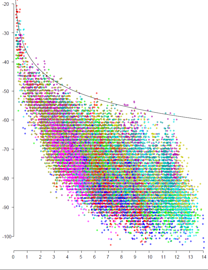
Why not just use the inverse-distance-squared law to estimate distance from the access point (AP)? The scattergram on the left shows about 20,000 RSS (Received Signal Strength) values (vertical axis, in dBm) versus actual distance between smartphone and access point (horizontal axis, in meters) in a typical three level house. The solid curve corresponds to the inverse square law — which is clearly not a good fit to the observed signal strength (other than providing an upper bound). More importantly, the spread in RSS for a given distance is huge, making inversion to estimate the distance from RSS ill posed. No path-loss model, no matter how complex, can overcome this problem.

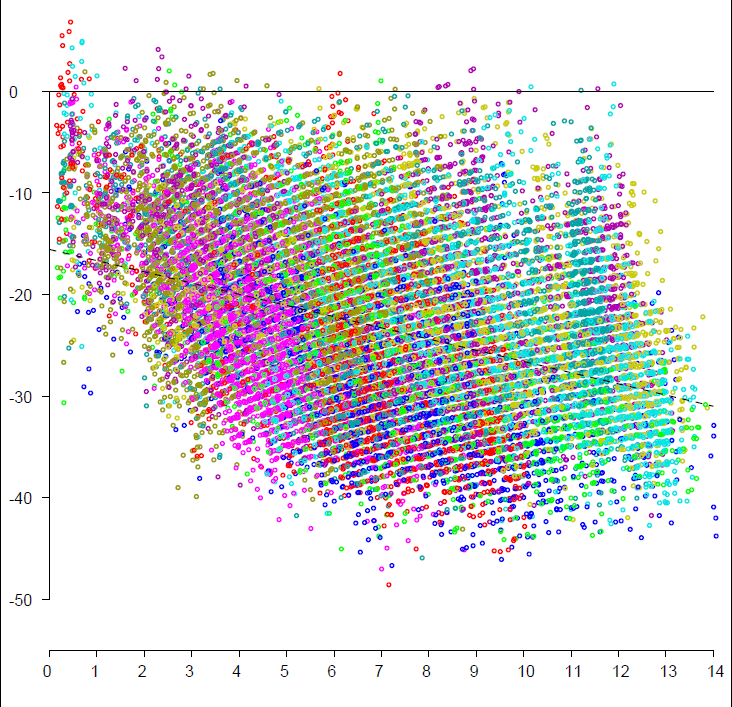
By the way, the observed decay with distance better fits that of a signal passing through an absorbing medium. If we subtract the expected inverse square drop off from the above, we are left with the scattergram on the right. An attempt to fit a linear relationship between excess path loss and distance leads to a slope of -1.1 dB per meter (although with a huge error term), as indicated by the dashed line.

Raleigh Fading, Rician Fading, Multi-path, Standing Waves, and more...

Still not convinced? Then look at this: The above “heat map” shows how signal strength in a multi-room apartment varies from place to place (floor plan shown on the right - for more details see Jason M. Cole's Helmhurts and also try his Helmhurts Android app ).

“Fingerprinting” RSSs

Since signal strength from a single source is so unhelpful in estimating distance, an alternate approach depends on signals from several APs and exploits the fact that different combinations of signal strengths from these APs will be found in different positions. This method requires first exploring the whole volume — and recording the RSS values for each of the APs in “each position.” In use, the position is then estimated from where the recorded RSSs best match the observed combination of RSSs. The “finger-printing” effort is one that has to be repeated when objects that may affect the RF field are moved. Or when the access point is moved slightly (to see how the RSS heat map changes dramatically with position of the source, click on the above heat map!).

Channel State Information (CSI)

RSS provides only one noisy estimate of the state of the channel. In orthogonal frequency-division multiplexing (OFDM) signalling, each subchannel has a state (amplitude and phase) given as a complex nummber. This state has to be estimated for proper decoding of the signal. The estimate is based on the received preamble. In the case of 20 MHz bandwidth, out of 64 subchannels, 52 are used for data, 4 for pilots and 8 are nulled. This means the CSI vector has 56 non-zero (complex) components, which provide much more information than the single (real) value of RSS does. Nevertheless, since using CSI requires a fingerprinting approach, it has the same disadvantages as the above. Further, Android does not make physical layer (PHY) information, such as the CSI, accessible to applications.

FTM RTT (802.11mc)

A much better way of estimating distance is FTM RTT as specified in IEEE 802.11mc (a.k.a. 802.11-2016)

Accessibility