Bayesian Grid

When it comes to recovering position from distance measurements, a good way of dealing with a probability distribution that can't be easily parameterized is to represent it with values on a regular grid. Shown above is a “heatmap” of the probability distribution on a grid superimposed on a floorplan. The stronger the red, the higher the probability that the initiator is there. Sequential Bayesian updates can be applied to such a grid of probabilities. This method starts with a prior distribution (perhaps uniform). A transition model is invoked at each step which modifies the distribution based on likely movement of the initiator (e.g. a random walk of a step size based on comfortable walking speed of 1.4 m/sec). If a floor plan is available, impenetrable walls can be taken into account in the transition model if desired. This is followed by Bayesian update based on FTM RTT distance measurements, which uses an observation model estimating the probability of seeing a measurement given the actual distance between a voxel and the responder.

FTM RTT distance measurement versus actual distance

Above is a histogram of the ratio of FTM RTT measurements and corresponding actual distances from over 20,000 results in a 3-story home of mostly wooden construction. Not unexpectedly, there is a strong bias for measurements to be larger than the actual distance - very few are smaller. In effect, the actual distance is a lower bound on the FTM RTT measurement (since nothing can travel faster than the speed of light). The measurement can be considerably larger than the actual distance because the signal may be slowed down by passing through building materials with large relative permittivity (see Measurement Errors). The dots in the figure are the actual histogram data, while the solid curve is a “double exponential” curve with a flat top. Note that the exponential drop is much slower on the right side than it is on the left.

Observation Model

Above is an observation model. Each curve is the conditional probability of observing a distance measurement (horizontal axis-meters) given a specific actual distance. Individual curves are shown for actual distances in 1 meter increments, starting at 1 meter. For details see the paper.

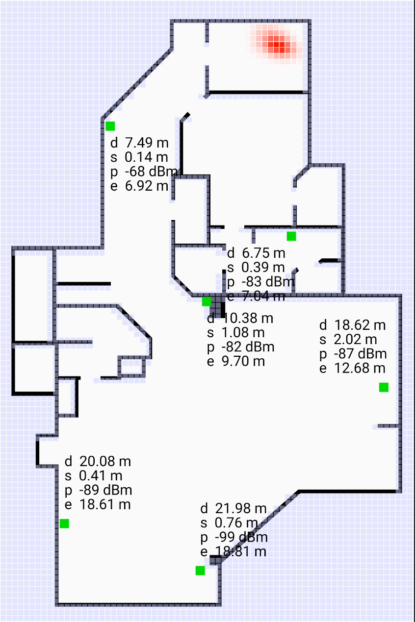
If a single position is required as output, rather than a distribution, one can, for example, use the mode (maximum likelihood) or the centroid (expected value) of the distibution.

As with other forms of “filtering”, there can be a lag in the response when the initiator moves more rapidly than the transition model expects. Also, a bad solution may get “trapped” behind walls, when a floor plan is used to prevent moving through walls in the transition model.

Accessibility