Peculiarities of FTM RTT Measurements — Position-Dependent Error
(Click on images to see larger versions).
 When the initiator and the responder are perfectly still,
with a clear line of sight,
measurements are deceptivitly stable and repeatable.
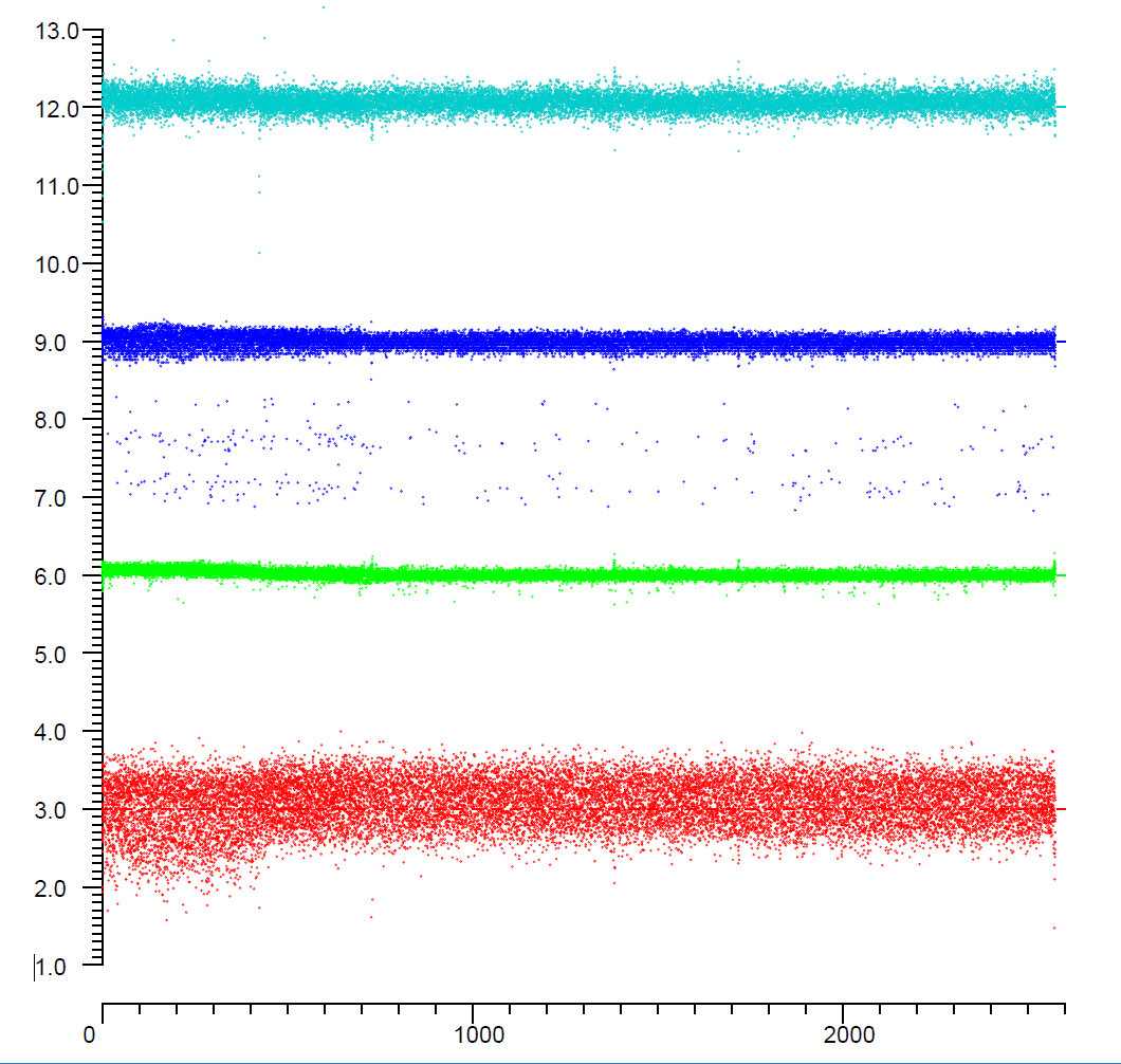
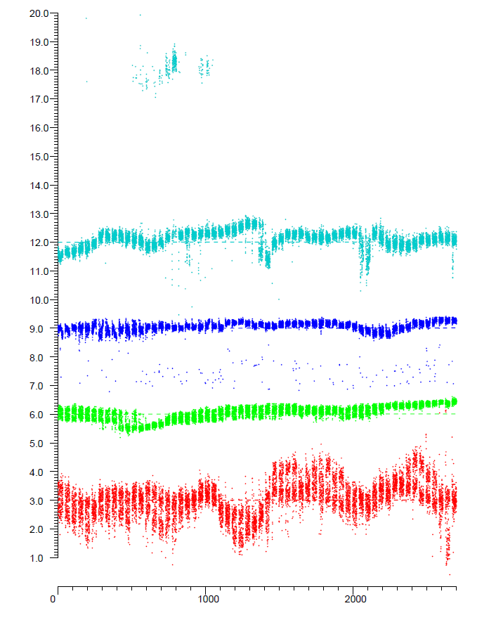
Shown in the above figure are traces for four different responders (color coded),
each of which is three meters from a stationary initiator,
over a period of about 45 minutes with sampling frequency of 8.5 Hz.
The horizontal axis is time in seconds and the vertical axis reported distance in meters
(The four plots are offset vertically from each other in 3 meter increments so as to avoid overlap).
There are obvious differences between the responders
The “red” responder, for example, has more
“noise” than the others,
while the “green” responder has
“measurement noise”
with standard deviation less than 0.2 meter.
The “blue” responder in this case has slightly higher
“noise” and shows some “outliers”
that are about 0.6, 1.2 or 1.9 meter too small.
Aside from that, one might conclude that these are all simply
measurements of stationary random processes with offsets and additive Gaussian
noise of magnitude that happens to be different for different responders.
When the initiator and the responder are perfectly still,
with a clear line of sight,
measurements are deceptivitly stable and repeatable.
Shown in the above figure are traces for four different responders (color coded),
each of which is three meters from a stationary initiator,
over a period of about 45 minutes with sampling frequency of 8.5 Hz.
The horizontal axis is time in seconds and the vertical axis reported distance in meters
(The four plots are offset vertically from each other in 3 meter increments so as to avoid overlap).
There are obvious differences between the responders
The “red” responder, for example, has more
“noise” than the others,
while the “green” responder has
“measurement noise”
with standard deviation less than 0.2 meter.
The “blue” responder in this case has slightly higher
“noise” and shows some “outliers”
that are about 0.6, 1.2 or 1.9 meter too small.
Aside from that, one might conclude that these are all simply
measurements of stationary random processes with offsets and additive Gaussian
noise of magnitude that happens to be different for different responders.
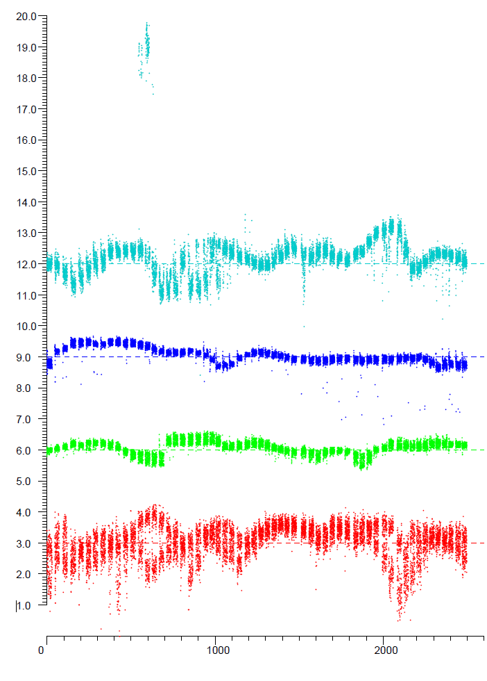
If the experiment is repeated at a different distance, again stable
results are obtained, although the errors in distance will be
different, and the “noise” will also change.
For example, the “blue”
responder may then have the same “noise” as the “green” responder.
And in some cases the “noise” becomes multimodal.
How exactly does the response depend on distance?
It turns out that we do not get very insightful results if we simply plot reported
distance versus actual distance while slowly varying the actual
distance. We get very “noisy” results that behave in
unexpected ways.
The reason for that may become clear after first considering the results of
step-wise distance changes:
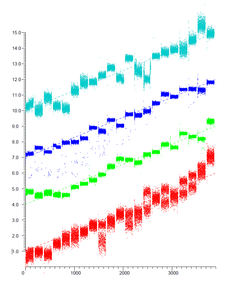 If we plot reported distance versus actual distance we get interesting and perhaps surprising results.
In the above plot, the initiator is moved in 250mm
steps relative to the same four responders, from 1 meter to 6 meter.
At each position, the response is again stable, but it does not
vary monotonically with actual distance.
Also, the “noise” is different for different distances,
and the distribution of readings for a given distance is not always unimodal.
If we plot reported distance versus actual distance we get interesting and perhaps surprising results.
In the above plot, the initiator is moved in 250mm
steps relative to the same four responders, from 1 meter to 6 meter.
At each position, the response is again stable, but it does not
vary monotonically with actual distance.
Also, the “noise” is different for different distances,
and the distribution of readings for a given distance is not always unimodal.
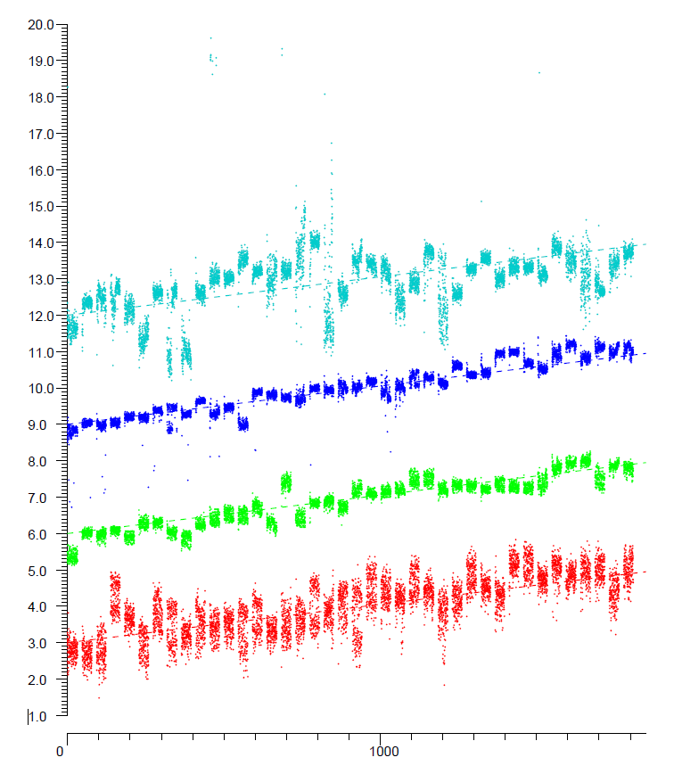 In an attempt to discover the “fine structure” of the dependence on
distance, the next plot (above) is for initiator positions that are
incremented in smaller steps, 50mm, from 3.0 meter to 4.95 meter.
Again, the reported distance is seen to be non-monotonic with actual
distance, and the distribution is sometimes multimodal.
Also, the “cyan” responder has some outliers were the reported
distance is about 6 meters too large.
In an attempt to discover the “fine structure” of the dependence on
distance, the next plot (above) is for initiator positions that are
incremented in smaller steps, 50mm, from 3.0 meter to 4.95 meter.
Again, the reported distance is seen to be non-monotonic with actual
distance, and the distribution is sometimes multimodal.
Also, the “cyan” responder has some outliers were the reported
distance is about 6 meters too large.
 Next,
we look at even finer intervals in distance to see whether some
underlying structure becomes apparent.
In the above plot, the initiator position is increment by 10mm,
from 3.0 meter to 3.39 meter.
Again, the reported distance is not monotonic with actual distance,
and the distribution is not always unimodal.
There is, however, starting to be just a hint at some coherence
in reported distance readings for neighboring (actual) distances.
Next,
we look at even finer intervals in distance to see whether some
underlying structure becomes apparent.
In the above plot, the initiator position is increment by 10mm,
from 3.0 meter to 3.39 meter.
Again, the reported distance is not monotonic with actual distance,
and the distribution is not always unimodal.
There is, however, starting to be just a hint at some coherence
in reported distance readings for neighboring (actual) distances.
 Finally, we use increments of just 2 mm (!), from 3.0 meter to 3.118 meter.
In the above plot more coherence starts to show itself.
Neighboring samples have somewhat similar properties.
So the finest spatial scale of the response pattern is surprisingly
small, namely a few millimeters.
Finally, we use increments of just 2 mm (!), from 3.0 meter to 3.118 meter.
In the above plot more coherence starts to show itself.
Neighboring samples have somewhat similar properties.
So the finest spatial scale of the response pattern is surprisingly
small, namely a few millimeters.
These plots show that the reported distance depends on the position in a
sensitive way — a movement of a just few millimeters can at
times produce a change of a meter in reported distance!
We call this “position-dependent error”.
Note also that the “noise” in the reported distance
varies sensitively with position — in some positions it can be
several times larger than it is in other positions.
It should be clear that the standard deviation of the
measurement in a fixed position (s.a. from the first plot above) is
not a useful measure of expected error in reported distance.
Correspondly, averaging a burst of FTM RTT “ping pong”
trial results is actually not all that useful in reducing the overall
measurement error (Android does 8 such trials at a time -
averaging 7 of them).
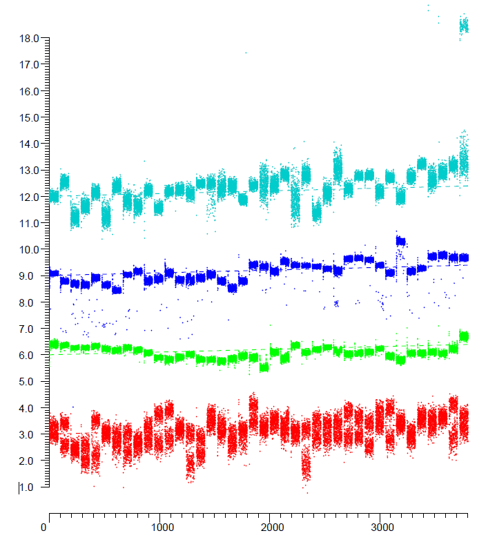
Moving across the line of sight
 What happens if we move orthogonal to the line of sight?
We might expect that the average measurements would not change.
As it turns out, they do change, but
perhaps a bit more slowly than they change with distance, as shown in the above plot,
where each step is 5mm across the line of sight, when the responders
are 3 meters from the initiator.
What happens if we move orthogonal to the line of sight?
We might expect that the average measurements would not change.
As it turns out, they do change, but
perhaps a bit more slowly than they change with distance, as shown in the above plot,
where each step is 5mm across the line of sight, when the responders
are 3 meters from the initiator.
How to make sense of all of this?
It appears that the error in the measured distance has a (small)
component of random “measurement noise,”
but that that is overshadowed by a much larger error that
depends on the position of the device.
We call this “position-dependent error”.
For a given position in space we obtain a certain fixed value,
plus a small amount of added random noise,
the magnitude of which also depends on position.
In some cases two (or more) values “compete” and we get a multi-modal distributions.
Importantly, the error in distance is much larger than the standard deviation
of the additive random noise.
This may all appear somewhat reminiscent of the need to have a rotating stage
in a microwave oven (which, by the way, operates at 2.4 GHz).
The RF field with standing waves due to reflection from the metal walls heats the food
in a spatially varying fashion, and to get more or less uniform
heating the food needs to be moved to sample this space of standing waves.
Yet, this analogy seems not to be entirely appropriate since
(i) the initiator and responder are not in a metallic box that would create standing waves,
but in relatively open space with a direct line of sight, and
(ii) the arrival of the first RF signal should not be affected
by RF energy that has travelled different, longer distances and arrives later
(except perhaps as a result of short-comings of the super-resolution
algorithms).
Some numbers of possible relevance:
- Wavelength in lower 5 GHz band: 57 mm, in upper 5 GHz band: 52 mm
- ADC sample period at 80 MSps is 12.5 nsec: equivalent to 3.75 m (round trip) or 1.875 m one way.
- Length of one OFDM symbol (plus cyclical prefix) 3.6 µsec: 1080 meter
- Wrap around of timing fields in FTM RTT (6 bytes, with 0.1 nsec resolution): 7.8 hours
Click here to go back to
main article on FTM RTT.
Berthold K.P. Horn,
bkph@ai.mit.edu
Accessibility