Introduction

Figure 1. Demo of our video super-resolution system.. For an input low-res video, our system is able to reconstruct its high-res by 4x up-sampling rate.

Multi-frame super resolution, namely estimating the high-res frames from a low-res sequence, is one of the fundamental problems in computer vision and has been extensively studied for decades. The problem becomes particularly interesting as high-definition devices such as HDTV's dominate the market. There is a great need for converting low-res, low-quality videos into high-res, noise-free videos that can be pleasantly viewed on HDTV's.

Although a lot of progress has been made in the past 30 years, super resolving real-world video sequences still remains an open problem. Most of the previous work assumes that the underlying motion has a simple parametric form, and/or that the blur kernel and noise levels are known. But in reality, the motion of objects and cameras can be arbitrary, the video may be contaminated with noise of unknown level, and motion blur and point spread functions can lead to an unknown blur kernel.

Therefore, a practical super resolution system should simultaneously estimate optical flow [Horn 1981], noise level [Liu 2008] and blur kernel [Kundur 1996] in addition to reconstructing the high-res frames. As each of these problems has been well studied in computer vision, it is natural to combine all these components in a single framework without making oversimplified assumptions.

In this paper, we propose a Bayesian framework for adaptive video super resolution that incorporates high-res image reconstruction, optical flow, noise level and blur kernel estimation. Using a sparsity prior for the high-res image, flow fields and blur kernel, we show that super resolution computation is reduced to each component problem when other factors are known, and the MAP inference iterates between optical flow, noise estimation, blur estimation and image reconstruction. As shown in Figure 1 and later examples, our system produces promising results on challenging real-world sequences despite various noise levels and blur kernels, accurately reconstructing both major structures and fine texture details. In-depth experiments demonstrate that our system outperforms the state-of-the-art super resolution systems [VH 2010, Shan 2008, Takeda 2009] on challenging real-world sequences.

A Bayesian Model

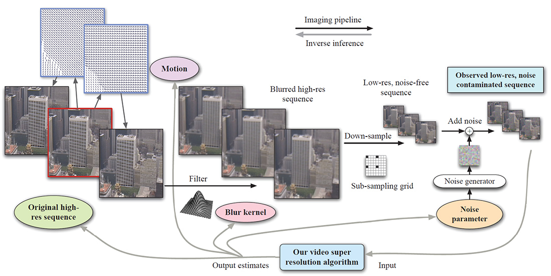
The imaging pipeline is shown in Figure 2, where the original high-res video sequence is generated by warping the high-res source frame (enclosed by a red rectangle) both forward and backward with some motion fields. The high-res sequence is then smoothed with a blur kernel, down-sampled and contaminated with noise to generate the observed sequence. Our adaptive video super resolution system not only estimates the high-res sequence, but also the underlying motion (on the lattice of original sequence), blur kernel and noise level.

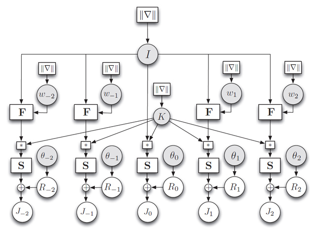
Figure 2 can be translated to the graphical model in Figure 3.

We use Bayesian maximum a posteriori (MAP) criterion to infer the optimum set of unknown variables

Where the posterior can be rewritten as the product of likelihood and prior

To deal with outliers, we assume an exponential distribution for the likelihood:

We use sparisty on derivatives to model the prior of the high-res image, flow field and blur kernel

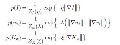
Naturally, the conjugae prior for the noise parameter θ_i is a Gamma distribution

Our optimization strategy is to fix three sets of parameters and estimate the other. It is straightforward to find that we indeed itereate the following four steps:

·  Image reconstruction: infer I

·  Motion estimation: infer {w_i}

·  Noise estimation: infer {θ_i}

·  Kernel estimation: infer K

It is clear that these four classical computer vision problems need to be solved simultaneously for video super resolution! The objective function has the form of L1 norm. We use iteratively reweighted least square (IRLS) to solve this convex optimization problem. The convergence procedure is shown in the following video, where the Itertion # shows the outer iteration where the four sets of variables are swept. IRLS # is the index of inner iteration where the high-res image gets optimized. Clearly, the images gets sharper as the algorithm progresses. In addition, the fact that the images gets dramatically sharper after the first outer iteration indicates that better estimates of motion, noise level and blur kernel lead to better estimate of the high-res image

Figure 4. Convergence of our system. You may want to play the video multiple times to see the optimization procedure.

Study on noise and blur

We collected 731 videos consisting of 102,206 frames as our database for the experiments. The videos are mostly of street scenes. One frame from each of the 731 videos was selected as the query image and histogram intersection matching was used to find its 20 nearest neighbors, excluding all other frames from the query video. The SIFT flow algorithm was then used to estimate the dense correspondence (represented as a pixel displacement field) between the query image and each of its neighbors. The best matches are the ones with the minimum energy.

Transition

To evaluate the matching obtained by SIFT flow, we performed a user study where we showed 11 users image pairs with 10 preselected sparse points in the first image and asked the users to select the corresponding points in the second image. This process is explained in Figure 12. The corresponding points selected by different users can vary, as shown on the right of Figure 13 . Therefore, we use the following metric to evaluate SIFT flow: for a pixel p, we have several human annotations zi as its flow vector, and w(p) as the estimated SIFT flow vector. We compute the probability of one human annotated flow is within distance r to SIFT flow w(p). This function of r is plotted on the left of Fig. 13 (red curve). For comparison, we plot the same probability function (blue curve) for minimum L1-norm SIFT matching, i.e. SIFT flow matching without spatial terms. Clearly, SIFT flow matches better to human annotation than minimum L1-norm SIFT matching.

Experimental Results

The goal is, given a single static image, to predict what motions are plausible in the image. This is similar to the recognition problem, but instead of assigning a label to each pixel, we want to assign possible motions.

City

We can zoom in and see the differences in details

Calendar

Street

Using the SIFT-based histogram matching, we can retrieve very similar video frames that are roughly spatially aligned. For common events such as cars moving forward on a street, the motion prediction can be quite accurate given enough samples in the database. We further refine the coarse motion prediction using the SIFT flow from the matched video frame to the query image. We use this correspondence to warp the temporally estimated motion of the retrieved video frame and hallucinate a motion field.

People

References

Last update: Aug, 2011