IEEE Transactions on Pattern Analysis and Machine Intelligence, Vol. 33, No. 5, 2011
SIFT Flow: Dense Correspondence across Scenes and its Applications
Ce Liu1 Jenny Yuen2 Antonio Torralba2
1Microsoft Research New England 2Massachusetts Institute of Techonolgy
Download SIFT flow Matlab/C++ code
Abstract |
|
| While image alignment has been studied in different areas of computer vision for decades, aligning images depicting different scenes remains a challenging problem. Analogous to optical flow where an image is aligned to its temporally adjacent frame, we propose SIFT flow, a method to align an image to its nearest neighbors in a large image corpus containing a variety of scenes. The SIFT flow algorithm consists of matching densely sampled, pixel-wise SIFT features between two images, while preserving spatial discontinuities. The SIFT features allow robust matching across different scene/object appearances, whereas the discontinuity preserving spatial model allows matching of objects located at different parts of the scene. Experiments show that the proposed approach robustly aligns complex scene pairs containing significant spatial differences. Based on SIFT flow, we propose an alignment based large database framework for image analysis and synthesis, where image information is transferred from the nearest neighbors to a query image according to the dense scene correspondence. This framework is demonstrated through concrete applications, such as motion field prediction from a single image, motion synthesis via object transfer, satellite image registration and face recognition. |
Introduction
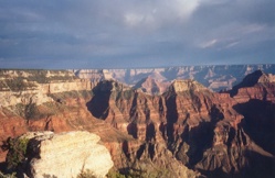
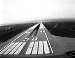
Image alignment, registration and correspondence are central topics in computer vision. There are several levels of scenarios in which image alignment dwells. The simplest level, aligning different views of the same scene, has been studied for the purpose of image stitching [1] and stereo matching [2], e.g. in Figure 1 (a). The considered transformations are relatively simple (e.g. parametric motion for image stitching and 1D disparity for stereo), and images to register are typically assumed to have the same pixel value after applying the geometric transformation.
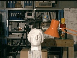
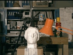
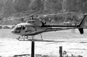
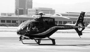
Image alignment becomes even more difficult in the object recognition scenario, where the goal is to align different instances of the same object category, as illustrated in Figure 1 (b). Sophisticated object representations [3] have been developed to cope with the variations of object shapes and appearances. However, these methods still typically require objects to be salient, similar, with limited background
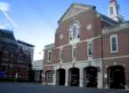
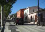
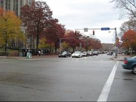
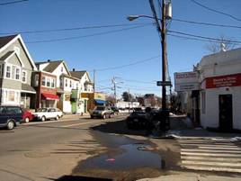
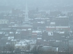
In this work, we are interested in a new, higher level of image alignment: aligning two images from different 3D scenes but sharing similar scene characteristics. Image alignment at the scene level is thus called scene alignment. As illustrated in Figure 1 (c), the two images to match may contain object instances captured from different viewpoints, placed at different spatial locations, or imaged at different scales. The two images may also contain different quantities of objects of the same category, and some objects present in one image might be missing in the other. Due to these issues the scene alignment problem is extremely challenging.
 |
 |
 |
 |
|
(a) Pixel level (stereo) |
(b) Object level (object recognition) |
|||
 |
 |
 |
 |
|
(i) Different perspectives and occlusions |
(ii) Multiple objects; no global transform |
|||
 |
 |
 |
 |
|
(iii) Background clutter |
(iv) High intra-class variations |
|||
(c) Scene level (scene alignment)
|
||||
Figure 1. Image alignment resides at
different levels. Researchers used to study image
alignment problems at the pixel
level, where two images are captured from the same scene with
slightly different time or at different perspectives [2] (a).
Recently, correspondence has been extended to the object level
(b) for object recognition [4]. We are interested in image
alignment at the scene level, where two images come from
different 3D scene but share similar scene characteristics (c).
SIFT flow is proposed to align the examples in (c) for scene
alignment
|
||||
Ideally, in scene alignment we want to build correspondence at the semantic level, i.e. matching at the object class level, such as buildings, windows and sky. However, current object detection and recognition techniques are not robust enough to detect and recognize all objects in images. Therefore, we take a different approach for scene alignment by matching local, salient, and transform-invariant image structures. We hope that semantically meaningful correspondences can be established through matching these image structures. Moreover, we want to have a simple, effective, object-free model to align image pairs such as the ones in Figure 1 (c).
Inspired by optical flow methods, which are able to produce dense, pixel-to-pixel correspondences between two images, we propose SIFT flow, adopting the computational framework of optical flow, but by matching SIFT descriptors instead of raw pixels. In SIFT flow, a SIFT descriptor [5] is extracted at each pixel to characterize local image structures and encode contextual information. A discrete, discontinuity preserving, flow estimation algorithm is used to match the SIFT descriptors between two images. The use of SIFT features allows robust matching across different scene/object appearances and the discontinuity-preserving spatial model allows matching of
Using SIFT flow, we propose an alignment-based large database framework for image analysis and synthesis. The information to infer for a query image is transferred from the nearest neighbors in a large database to this query image according to the dense scene correspondence estimated by SIFT flow. Under this framework, we apply SIFT flow to two novel applications: motion prediction from a single static image, where a motion field is hallucinated from a large database of videos, and motion transfer, where a still image is animated using object motions transferred from a similar moving scene. We also apply SIFT flow back to the regime of traditional image alignment, such as satellite image registration and face recognition. Through these examples we demonstrate the potential of SIFT flow for broad applications in computer vision and computer graphics.
SIFT flow algorithm
Dense SIFT descriptor and visualization
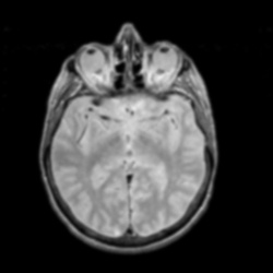
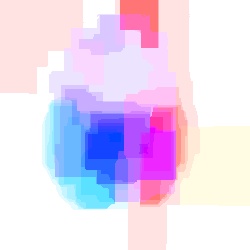
SIFT is a local descriptor to characterize local gradient information [5]. In [5], SIFT descriptor is a sparse feature epresentation that consists of both feature extraction and detection. In this paper, however, we only use the feature extraction component. For every pixel in an image, we divide its neighborhood (e.g. 16×16) into a 4×4 cell array, quantize the orientation into 8 bins in each cell, and obtain a 4×4×8=128-dimensional vector as the SIFT representation for a pixel. We call this per-pixel SIFT descriptor SIFT image.
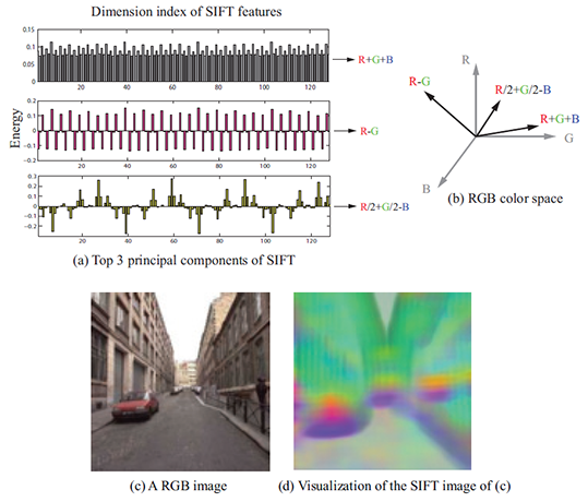
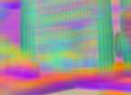
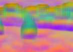
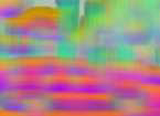
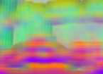
To visualize SIFT images, we compute the top three principal components of SIFT descriptors from a set of images, and then map these principal components to the principal components of the RGB space, as shown in Figure 2. Via projection of a 128D SIFT descriptor to a 3D subspace, we are able to compute the SIFT image from an RGB image in Figure 2 (c) and visualize it in (d). In this visualization, the pixels that have similar color may imply that they share similar local image structures. Note that this projection is only for visualization; in SIFT flow, the entire 128 dimensions are used for matching.
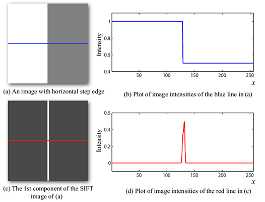
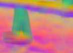
Notice that even though this SIFT visualization may look blurry as shown in Figure 2 (d), SIFT images indeed have high spatial resolution as suggested by Figure 3. We designed an image with a horizontal step-edge (Figure 3 (a)), and show the 1st component of the SIFT image of (a) in (c). Because every row is the same in (a) and (c), we plot the middle row of (a) and (c) in (b) and (d), respectively. Clearly, the SIFT image contains a sharp edge with respect to the sharp edge in the original image.
|
|
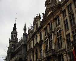
| Figure 2. Visualization of SIFT images. To visualize SIFT images, we compute the top three principal components of SIFT descriptors from a set of images (a), and then map these principal components to the principal components of the RGB space (b). For an image in (c), we compute the 128-d SIFT feature for every pixel, project the SIFT feature to 3d color space, and visualize the SIFT image as shown in (d). Intuitively, pixels with similar colors share similar structures. | Figure 3. The resolution of SIFT images. Although histograms are used to represent SIFT features, SIFT images are able to capture image details. For a toy image with a horizontal stepedge in (a), we show the 1st component of the SIFT image in (c).We plot the slice of a horizontal line in (a) (blue) and (c) (red) in (b) and (d), respectively. The sharp boundary in (d) suggests that SIFT images have high resolutions. |
Matching Objective
We formulate SIFT flow the same as optical flow with the exception of matching SIFT descriptors instead of RGB values. Therefore, the objective function of SIFT flow is very similar to that of optical flow. Let p=(x,y) be the grid coordinate of images, and w(p)=(u(p),v(p)) be the flow vector at p. We only allow u(p) and v(p) to be integers and we assume that there are L possible states for u(p) and v(p), respectively. Let s1 and s2 be two SIFT images that we want to match. Set ε contains all the spatial neighborhoods (a four-neighbor system is used). The energy function for SIFT flow is defined as:
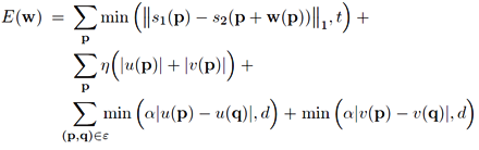
which contains a data term, small displacement term and smoothness term (a.k.a. spatial regularization). The data term on line 1 constrains the SIFT descriptors to be matched along with the flow vector w(p). The small displacement term on line 2 constrains the flow vectors to be as small as possible when no other information is available. The smoothness term on line 3 constrains the flow vectors of adjacent pixels to be similar. In this objective function, truncated L1 norms are used in both the data term and the smoothness term to account for matching outliers and flow discontinuities, with t and d as the threshold, respectively.
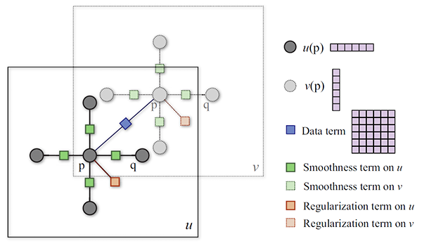
We use a dual-layer loopy belief propagation as the base algorithm to optimize the objective function. Different from the usual formulation of optical flow [6], the smoothness term in the above equation is decoupled, which allows us to separate the horizontal flow u(p) from the vertical flow v(p) in message passing, as suggested by [7]. As a result, the complexity of the algorithm is reduced from O(L4) to O(L2) at one iteration of message passing. The factor graph of our model is shown in Figure 4. We set up a horizontal layer u and vertical layer v with exactly the same grid, with the data term connecting pixels at the same location. In message passing, we first update intra-layer messages in u and v separately, and then update inter-layer messages between u and v. Because the functional form of the objective function has truncated L1 norms, we use distance transform function [8] to further reduce the complexity, and sequential belief propagation (BP-S) [9] for better convergence.
|
|

Coarse-to-fine matching scheme
Despite the speed up, directly optimizing the objective function using dual-layer belief propagation scales poorly with respect to image dimension. In SIFT flow, a pixel in one image can literally match to any pixels in the other image. Suppose the image has h2 pixels, then L ≈ h, and the time and space complexity of this dual-layer BP is O(h4). For example, the computation time for 145×105 images with an 80×80 search window is 50 seconds. It would require more than two hours to process a pair of 256×256 images with a memory usage of 16GB to store the data term
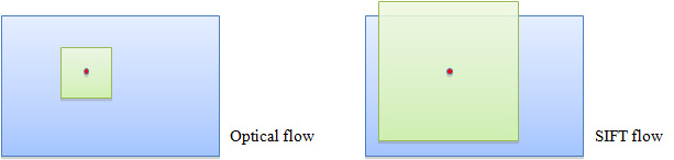 |
Figure 6. One big
difference between optical flow and SIFT flow is that the search
window size for SIFT flow is much larger since an object can
move drastically from one image to another in scene alignment.
Therefore, we need to design efficient algorithm to cope with
the complexity. |
To address the performance drawback, we designed a coarse-to-fine SIFT flow matching scheme that significantly improves the performance. The basic idea is to roughly estimate the flow at a coarse level of image grid, then gradually propagate and refine the flow from coarse to fine. The procedure is illustrated in Figure 6. For simplicity, we use s to represent both s1 and s1. A SIFT pyramid {s(k)} is established, where s(1) = s and s(k+1) is smoothed and downsampled from s(k). At each pyramid level k, let pk be the coordinate of the pixel to match, ck be the offset or centroid of the searching window, and w(pk) be the best match from BP. At the top pyramid level s(3), the searching window is centered at p3 (c3=p3) with size m×m, where m is the width (height) of s(3). The complexity of BP at this level is O(m4). After BP converges, the system propagates the optimized flow vector w(p3) to the next (finer) level to be c2 where the searching window of p2 is centered. The size of this searching window is fixed to be n×n with n=11. This procedure iterates from s(3) to s(1) until the flow vector w(p1) is estimated. The complexity of this coarse-to-fine algorithm is O(h2 log h), a significant speed up compared to O(h4). Moreover, we double η and retain α and d as the algorithm moves to a higher level of pyramid in the energy minimization. Using the proposed coarse-to-fine matching scheme and modified distance transform function, the matching between two 256×256 images takes 31 seconds on a workstation with two quad-core 2.67 GHz Intel Xeon CPUs and 32 GB memory, in a C++ implementation.
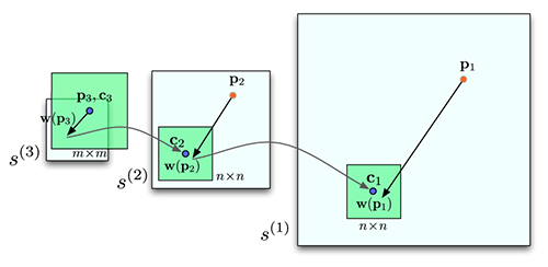 |
Figure 7. An
illustration of coarse-to-fine SIFT flow matching on pyramid.
The green square is the searching window for pk at each pyramid
level k. For simplicity only one image is shown here,
where pk is on image s1, and ck and w(pk) are on image
s2. |
A natural question is whether the coarse-to-fine matching scheme can achieve the same minimum energy as the ordinary matching scheme (using only one level).We randomly selected 200 pairs of images to estimate SIFT flow, and check the minimum energy obtained using coarse-to-fine scheme and ordinary scheme (non coarse-to-fine), respectively. For these 256 × 256 images, the average running time of coarse-tofine SIFT flow is 31 seconds, compared to 127 minutes in average for the ordinary matching. The coarse-to-fine scheme not only runs significantly faster, but also achieves lower energies most of the time compared to the ordinary matching algorithm as shown in Figure 8. This is consistent with what has been discovered in the optical flow community: coarse-tofine search not only speeds up computation but also leads to better solutions.
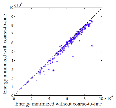 |
Figure 8. Coarse-to-fine SIFT flow not only runs significantly
faster, but also achieves lower energies most of the time. Here
we compare the energy minimized using the coarse-to-fine
algorithm (y-axis) and using the single-level version (x-axis) by
running them on 200 pairs of examples. The coarse-to fine
matching achieves a lower energies compared to the ordinary
matching algorithm most of the time. |
Neighborhood of SIFT flow
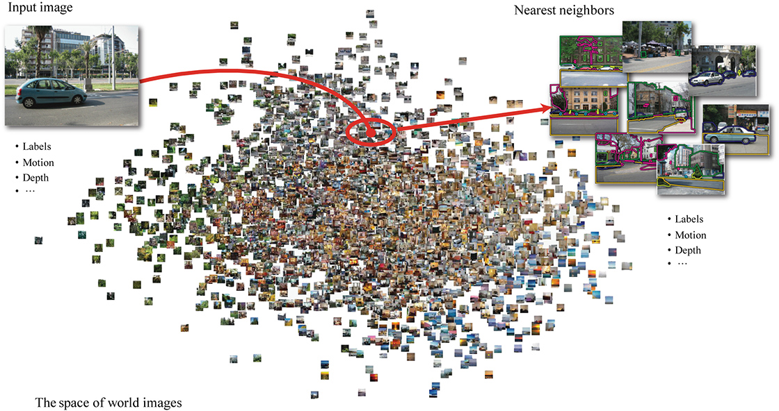
In theory, we can apply optical flow to two arbitrary images to estimate a correspondence, but we may not get a meaningful correspondence if the two images are from different scene categories. In fact, even when we apply optical flow to two adjacent frames in a video sequence, we assume dense sampling in time so that there is significant overlap between two neighboring frames. Similarly, in SIFT flow, we define the neighborhood of an image as the nearest neighbors when we query a large database with the input. Ideally, if the database is large and dense enough to contain almost every possible image in the world, the nearest neighbors will be close to the query image, sharing similar local structures. This motivates the following analogy with optical flow:
|
As dense sampling of the time domain is assumed to enable tracking, dense sampling in (some portion of) the space of world images is assumed to enable scene alignment. For a query image, we use a fast indexing technique to retrieve its nearest neighbors that will be further aligned using SIFT flow. As a fast search we use spatial histogram matching of quantized SIFT features [11]. First, we build a dictionary of 500 visual words [12] by running K-means on 5000 SIFT descriptors randomly selected out of all the video frames in our dataset. Then, histograms of the visual words are obtained on a two-level spatial pyramid [13], [11], and histogram intersection is used to measure the similarity between two images.
Experiments
Video retrieval results
We collected 731 videos consisting of 102,206 frames as our database for the experiments. The videos are mostly of street scenes. One frame from each of the 731 videos was selected as the query image and histogram intersection matching was used to find its 20 nearest neighbors, excluding all other frames from the query video. The SIFT flow algorithm was then used to estimate the dense correspondence (represented as a pixel displacement field) between the query image and each of its neighbors. The best matches are the ones with the minimum energy.
|
||||||||||||||
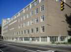
|
In this example, SIFT flow reshuffles the windows in the best match image to match the query. |
||||||||||||||
|
||||||||||||||
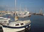
|
SIFT flow repositions and rescales the sailboat in the best match image to match the query. Notice that not only the foreground objects, but also the background pixels are aligned in SIFT flow. |
||||||||||||||
|
||||||||||||||
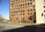
|
For this example, SIFT flow hallucinated a third window from the taxi to match the input SUV. Again, not only are the foreground objects aligned, but also the background objects. It shows the power of dense correspondence. |
||||||||||||||
|
||||||||||||||
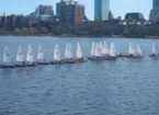
|
SIFT flow can also deal with multiple objects. In this example, SIFT flow reproduced and rearranged the sailboats in the best match to align to the query. |
||||||||||||||
|
||||||||||||||
|
For these two example where the correspondence is not obvious to humans, SIFT flow is able to find a reasonable correspondence that aligns these two very different houses. |
||||||||||||||
|
||||||||||||||
|
Since there is only one sequence of clock in our database, SIFT flow can only find an elevator door as the best match to the query, by breaking the rectangular structure and reforming it to form a circle.
|
||||||||||||||
|
Figure 10. Some typical SIFT flow retrieving/matching examples.
|


Ranking improvement
|
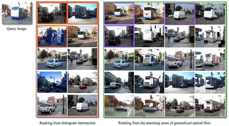
| Figure 11. SIFT flow typically improves ranking of the nearest neighbors. Images enclosed by the red rectangle (middle) are the top 10 nearest neighbors found by histogram intersection, displayed in scan-line order (left to right, top to bottom). The top three nearest neighbors are enclosed by orange. Images enclosed by the green rectangle are the top 10 nearest neighbors ranked by the minimum energy obtained by SIFT flow, and the top three nearest neighbors are enclosed by purple. The warped nearest neighbor image is displayed to the right of the original image. Note how the retrieved images are re-ranked according to the size of the depicted vehicle by matching the size of the bus in the query. |
SIFT flow evaluation
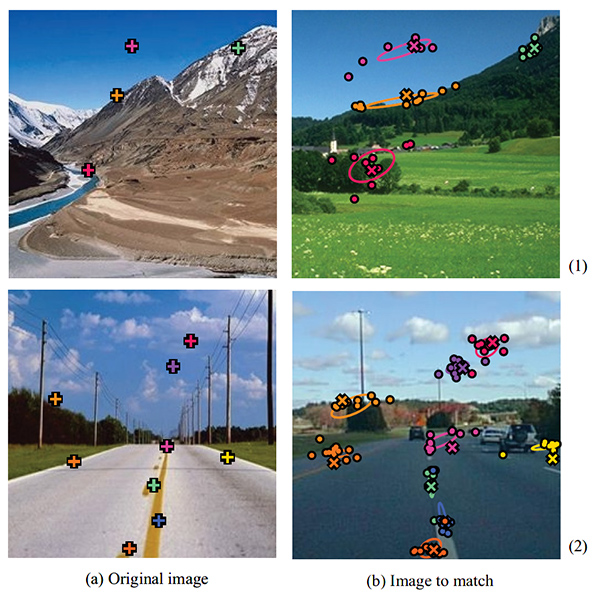
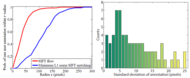
To evaluate the matching obtained by SIFT flow, we performed a user study where we showed 11 users image pairs with 10 preselected sparse points in the first image and asked the users to select the corresponding points in the second image. This process is explained in Figure 12. The corresponding points selected by different users can vary, as shown on the right of Figure 13 . Therefore, we use the following metric to evaluate SIFT flow: for a pixel p, we have several human annotations zi as its flow vector, and w(p) as the estimated SIFT flow vector. We compute the probability of one human annotated flow is within distance r to SIFT flow w(p). This function of r is plotted on the left of Fig. 13 (red curve). For comparison, we plot the same probability function (blue curve) for minimum L1-norm SIFT matching, i.e. SIFT flow matching without spatial terms. Clearly, SIFT flow matches better to human annotation than minimum L1-norm SIFT matching.
|
| Figure 12. For an image pair such as row (1) or row (2), a user defines several sparse points in (a) as “+”. The human annotated matchings are marked as dot in (b), from which a Gaussian distribution is estimated and displayed as an ellipse. The correspondence estimated from SIFT flow is marked as “×” in (b). |
|
| Figure 13. The evaluation of SIFT flow using human annotation. Left: the probability of one human annotated flow lies within r distance to the SIFT flow as a function of r (red curve). For comparison, we plot the same probability for direct minimum L1-norm matching (blue curve). Clearly, SIFT flow matches human perception better. Right: the histogram of the standard deviation of human annotation. Human perception of scene correspondence varies from subject to subject. |
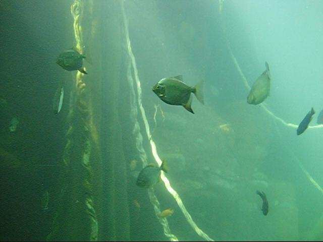
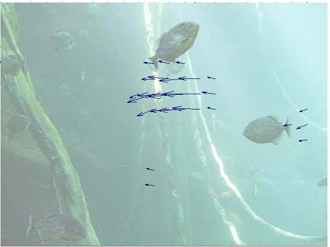
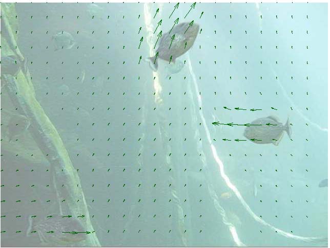
Motion hallucination
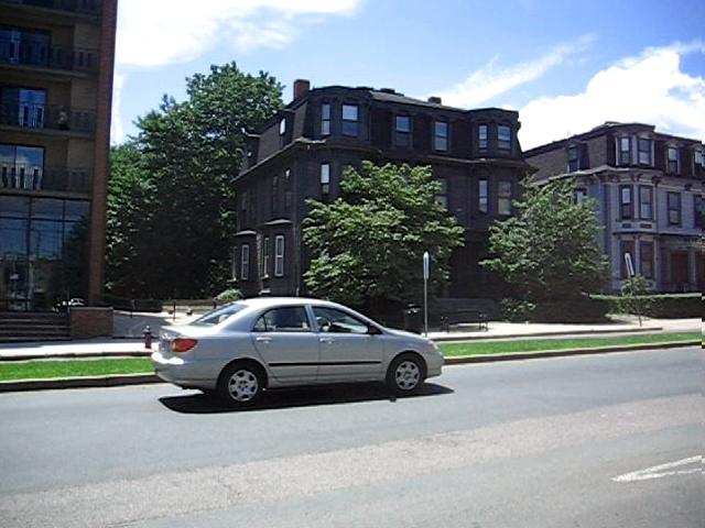
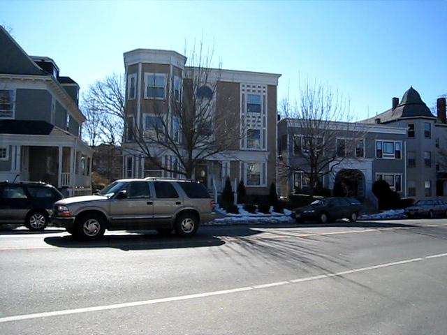
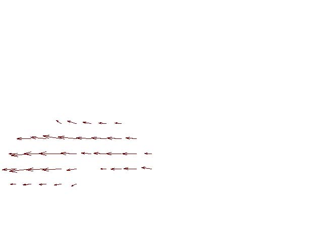
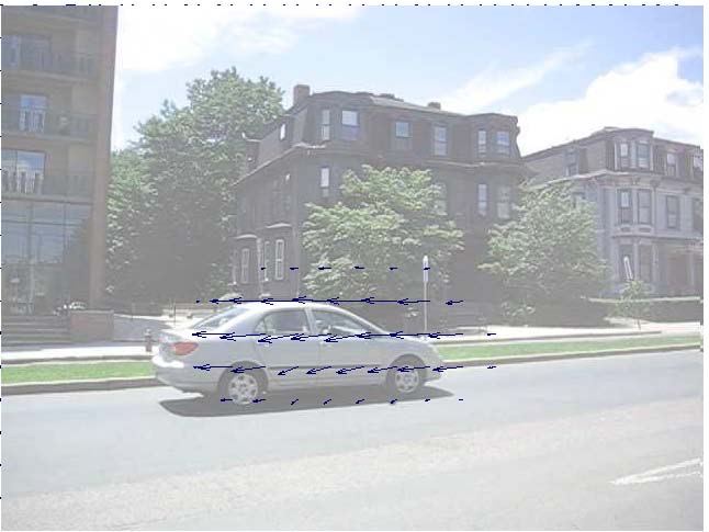
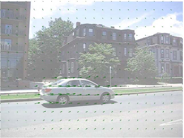
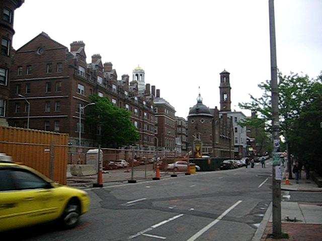
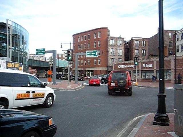
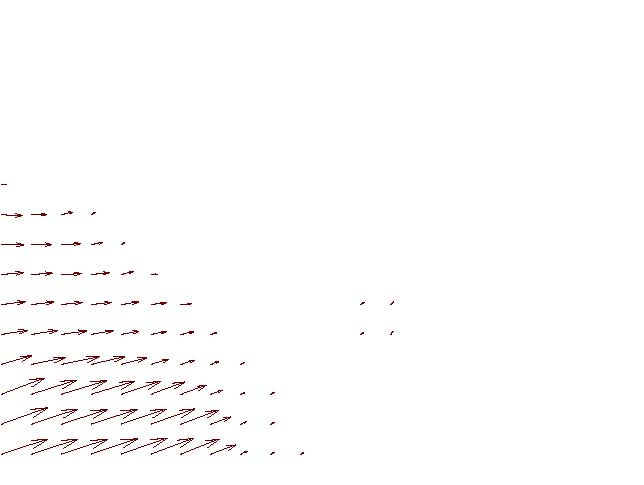
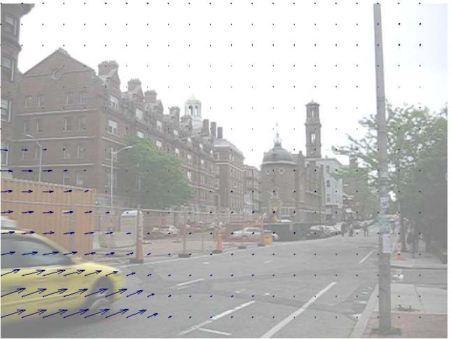
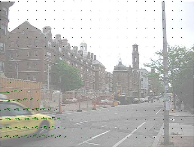
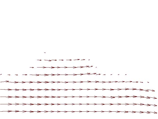
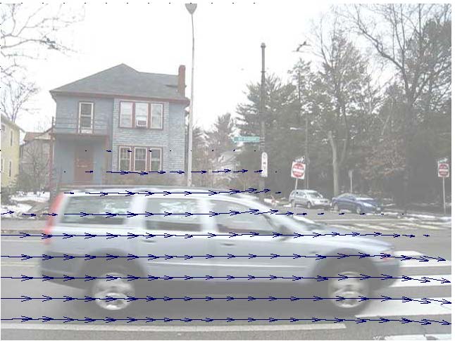
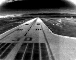
Predict motion fields from a single image
The goal is, given a single static image, to predict what motions are plausible in the image. This is similar to the recognition problem, but instead of assigning a label to each pixel, we want to assign possible motions.
Using the SIFT-based histogram matching, we can retrieve very similar video frames that are roughly spatially aligned. For common events such as cars moving forward on a street, the motion prediction can be quite accurate given enough samples in the database. We further refine the coarse motion prediction using the SIFT flow from the matched video frame to the query image. We use this correspondence to warp the temporally estimated motion of the retrieved video frame and hallucinate a motion field.
 |
 |
 |
 |
 |
 |
 |
 |
 |
 |
 |
 |
 |
 |
 |
 |
 |
 |
 |
 |
 |
 |
 |
 |
 |
Original Image |
Database match |
Motion of database match |
Warped and transferred motion |
Ground truth of original |
| Figure 14. Motion from a single image. (a) Original image; (b) bast match in the video database; (c) temporal motion field of (b); (d) warped motion of (c) and superimposed on (a), according to the estimated SIFT flow; (e) the “ground truth” temporal motion of (a) (estimated from the video containing (a)). The predicted motion is based on the motion present in other videos with image content similar to the query image. | ||||
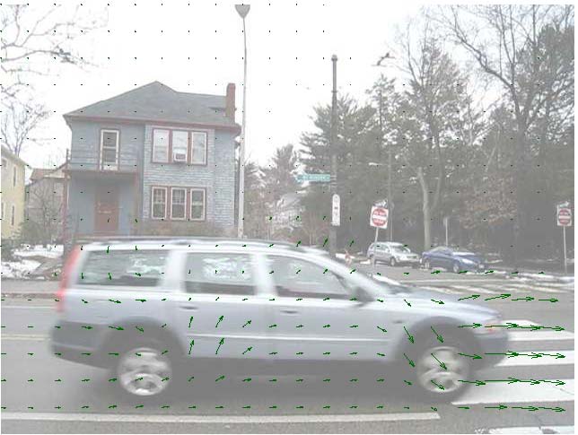
While there are many improbable flow fields (e.g. a car moving upwards), each image can have multiple plausible motions : a car or a boat can move
forward, in reverse, turn, or remain static:
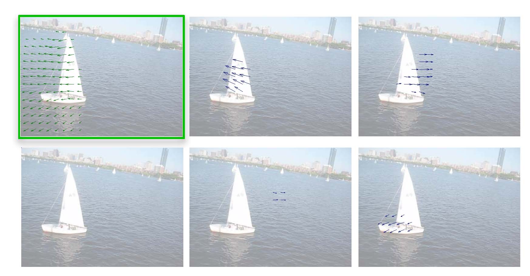 |
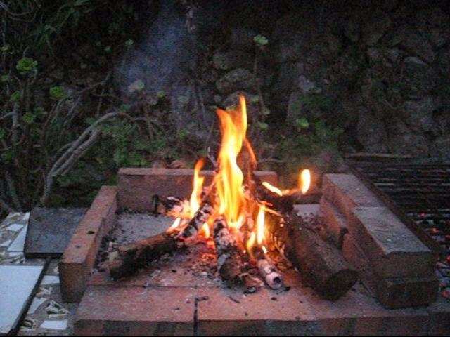
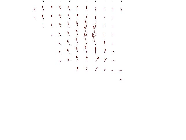
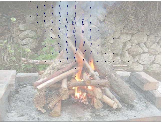
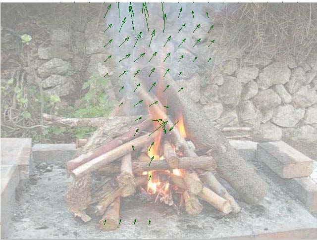
Figure 15. A still query image with its temporally estimated motion field (in the green frame) and multiple motion fields predicted by
motion transfer from a large video database. |
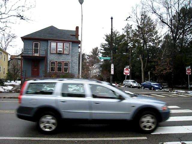
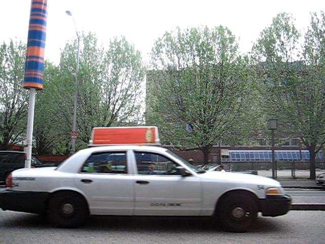
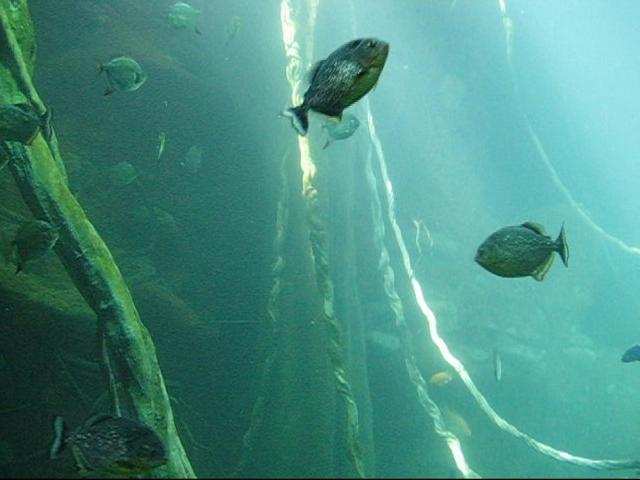
Motion synthesis via moving objects transfer
Given a still image, our system retrieves a video that matches the scene the best. Since the scenes are already aligned, the moving objects in the video already have the correct size, orientation, and lighting to fit in the still image. The third column shows synthesized video created by transferring the moving pixels from the video to the still image. Click on the thumbnails to show the videos.
 |
 |
 |
 |
 |
 |
 |
 |
 |
(a) Still query image
|
(b) Database video retrieval
|
(c) Composite video
|
| Figure 16. Motion synthesis via object transfer. Query images (a), the top video match (b), and the synthesized sequence (c) obtained by transferring the moving objects from the video to the still query image. | ||
Image registration
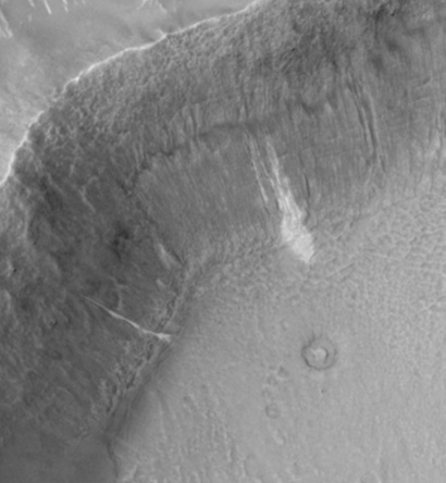
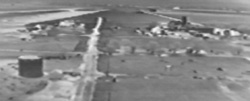
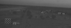
SIFT flow can be used to align images of very different texture and appearances. One example is to align two Mars images below. These two images look similar, but it's difficult to align them because of the change of local image difference and global distortions. But SIFT flow is able to align the two images well and to discover the cease that splits the land.
 |
 |
 |
| (a) Image 1 | (b) Image 2 | (c) Sparse feature matching |
 |
 |
 |
| (e) Flipping image 1 and warped image 2 | (f) Estimated SIFT flow field | (g) Flow discontinuities with the original images |
| Figure 17. SIFT flow can be applied to align satellite images. The two Mars satellite images (a) and (b) taken four years apart, show different local appearances. The result of sparse feature detection and matching is shown in (c), whereas the results of SIFT flow are displayed in (e) to (f). We super-impose the discontinuities from the estimated SIFT flow field in (f) to the original two frames and display the animation in (g). | ||
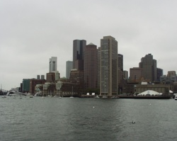
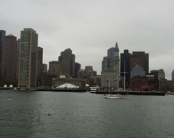
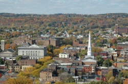
We then moved to the earth. We cropped two satellite pictures of MIT from Google Map and Microsoft Virtual Earth, respectively, and we applied SIFT flow to align these two images. Even though the two pictures were taken at different seaons and different time of a day (check the difference of the trees and shadows), our algorithm successfully uncovered the underneath geometric transform.
 |
 |
 |
| (a) Before alignment | (b) After alignment | (b) Estimated flow field |
| Figure 18. SIFT flow is applied to align two aerial images of MIT campus. | ||
We also tested SIFT flow on some challenging examples from http://www.vision.cs.rpi.edu/gdbicp/dataset/ [14]. Notice that SIFT flow is NOT specially designed for the senario considered in their work, e.g. little overlap, rigid geometric transform. But our algorithm does a pretty good job. The same parameter setting is used for generating the following results. SIFT flow failed to uncover the right transform for the bottom two examples because the two input images are too different with little overlap.
(a) Image 1 |
(b) Image 2 |
(c) Flipping betwee image 1 and warped image 2 |
(d) Flow field (hue indicates orientation and saturation indicates magnitude) |
 |
 |
 |
 |
 |
 |
 |
 |
 |
 |
 |
 |
 |
 |
 |
 |
 |
 |
 |
 |
 |
 |
 |
 |
 |
 |
 |
 |
 |
 |
 |
 |
 |
 |
 |
 |
 |
 |
 |
 |
(a) Image 1 |
(b) Image 2 |
(c) Flipping betwee image 1 and warped image 2 |
(d) sFlow field (hue indicates orientation and saturation indicates magnitude) |
| Figure 19. SIFT flow can be applied to same-scene image registration but under different lighting and imaging conditions. Column (a) and (b) are some examples from [14]. Column (c) is the estimated SIFT flow field, (d) is the warped image 2. | |||
Face recognition
Aligning images with respect to structural image information contributes to building robust visual recognition systems. We design a generic image recognition framework based on SIFT flow and apply it to face recognition, since face recognition can be a challenging problem when there are large pose and lighting variations in large corpora of subjects.
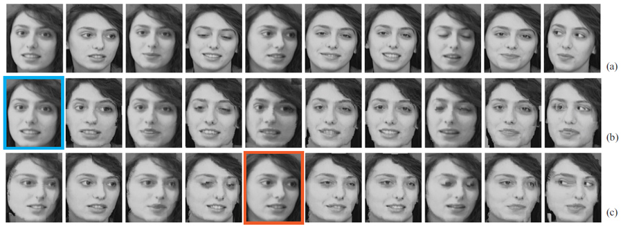
We use the ORL database [15] for this experiment. This database contains a total of 40 subjects and 10 images with some pose and expression variation per subject. In Fig. 23, a female sample is selected as an example to demonstrate how dense registration can deal with pose and expression variations. We first select the first image as the query, apply SIFT flow to align the rest of the images to the query, and display the warped images with respect to the SIFT flow field in Figure 20 (b). Notice how the poses and expressions of other images are rectified to that of the query. We can also choose a different sample as query and align the rest of the images to this query, as demonstrated in (c). Distances established on images after the alignment will be more meaningful than the distances directly on the original images.
|
| Figure 20. SIFT flow can account for pose, expression and lighting changes for face recognition. (a): Ten samples of one subject in ORL database [15]. Notice pose and expression variations of these samples. (b): We select the first image as the query, apply SIFT flow to align the rest of the images to the query, and display the warped images with respect to the dense correspondence. The poses and expressions are rectified to that of the query after the warping. (c): The same as (b) except for choosing the fifth sample as the query. |
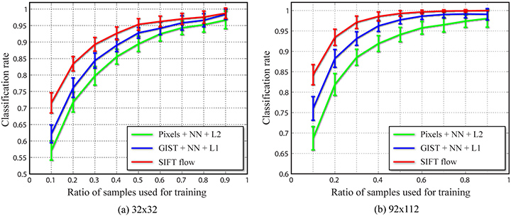
In order to compare with the state of the art, we conducted experiments for both original size (92×112) and downsampled (32×32) images. We randomly split a γ (γ ∈(0, 1)) portion of the samples for each subject for training, and use the rest 1−γ portion for testing. For each test image, we first retrieve the top nearest neighbors (maximum 20) from the training database using GIST matching [16], and then apply SIFT flow to find the dense correspondence from the test to each of its nearest neighbors by optimizing the SIFT flow objective. We assign the subject identity associated with the best match, i.e. the match with the minimum matching objective, to the test image. In other words, this is a nearest neighbor approach where the SIFT flow score is as the distance metric for object recognition.
|
| Figure 21. SIFT flow is applied for face recognition. The curves in (a) and (b) are the performance plots for low-res and highres images in the ORL face database, respectively. SIFT flow significantly boosted the recognition rate especially when there are not enough training samples |
The experimental results are shown in Figure 24. We use the nearest neighbor classifier based on pixel-level Euclidean distance (Pixels + NN + L2) and nearest neighbor classifier using the L1-norm distance on GIST [16] features (GIST + NN + L1) as the benchmark. Clearly, GIST features outperform raw pixel values since GIST feature is invariant to lighting changes. SIFT flow further improves the performance as SIFT flow is able to align images across different poses. We observe that SIFT flow boosts the classification rate significantly especially when there are not enough samples (small γ). We compare the performance of SIFT flow with the state of the art [17], where facial components are explicitly detected and aligned. The results of few training samples are listed in Table 1. Our recognition system based on SIFT flow is comparable with the state of the art when there are very few samples for training.
| Test errors | 1 training sample | 2 training samples | 3 training samples |
| S-LDA[17] | N/A | 17.1±2.7 | 8.1±1.8 |
| SIFT flow | 28.4 | 16.6±2.2 | 8.9±2.1 |
|
Table 1. Our face recognition system using SIFT flow is comparable with
the state of the art [17] when there are only few (one or two)
training samples. |
|||
Alignment-based framework
Using SIFT flow as a tool for scene alignment, we designed an alignment-based large database framework for image analysis and synthesis, as illustrated in Figure 22. For a query image, we retrieve a set of nearest neighbors in the database and transfer information such as motion, geometry and labels from the nearest neighbors to the query. This framework is concretely implemented in motion prediction from a single image, motion synthesis via object transfer and face recognition. In [18], the same framework was applied for object recognition and scene parsing. Although large-database frameworks have been used before in visual recognition [19] and image editing [20], the dense scene alignment component of our framework allows greater flexibility for information transfer in limited data scenarios.
|
| Figure 22. An alignment-based large database framework for image analysis and synthesis. Under this framework, an input image is processed by retrieving its nearest neighbors and transferring their information according to some dense scene correspondence. |
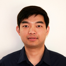
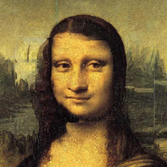
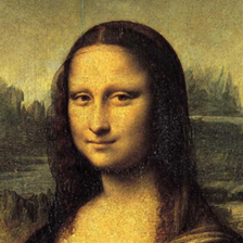
What is there is no training data? Well, we can still use our SIFT flow algorithm for fun. I (Ce Liu) always wonder how Leonard da Vinci would like to portrait me. Although we live in different eras, SIFT flow helps to imagine what he would draw (in the middle). :)
 |
 |
 |
References
| [1] | R. Szeliski. Image alignment and stiching: A tutorial. Foundations and Trends in Computer Graphics and Computer Vision, 2(1), 2006. |
| [2] | D. Scharstein and R. Szeliski. A taxonomy and evaluation of dense two-frame stereo correspondence algorithms. IJCV, 47(1):7–42, 2002. |
| [3] | S. Belongie, J. Malik, and J. Puzicha. Shape context: A new descriptor for shape matching and object recognition. NIPS, 2000. |
| [4] | A. Berg, T. Berg., and J. Malik. Shape matching and object recognition using low distortion correspondence. CVPR, 2005. |
| [5] | D. G. Lowe. Object recognition from local scale-invariant features. ICCV, pages 1150–1157, Kerkyra, Greece, 1999. |
| [6] | T. Brox, A. Bruhn, N. Papenberg, and J. Weickert. High accuracy optical flow estimation based on a theory for warping. ECCV, pages 25–36, 2004. |
| [7] | A. Shekhovtsov, I. Kovtun, and V. Hlavac. CVPR, 2007. |
| [8] | P. F. Felzenszwalb and D. P. Huttenlocher. IJCV, 70(1):41–54, 2006. |
| [9] | R. Szeliski, R. Zabih, D. Scharstein, O. Veksler, V. Kolmogorov, A. Agarwala, M. Tappen, and C. Rother. A comparative study of energy minimization methods for markov random fields with smoothness-based priors. TPAMI, 30(6):1068–1080, 2008. |
| [10] | S. Baker, D. Scharstein, J. P. Lewis, S. Roth, M. J. Black, and R. Szeliski. A database and evaluation methodology for optical flow. ICCV, 2007. |
| [11] | S. Lazebnik, C. Schmid, and J. Ponce. Beyond bags of features: Spatial pyramid matching for recognizing natural scene categories. CVPR, volume II, pages 2169–2178, 2006. |
| [12] | J. Sivic and A. Zisserman. Video Google: a text retrieval approach to object matching in videos. ICCV, 2003. |
| [13] | K. Grauman and T. Darrell. Pyramid match kernels: Discriminative classification with sets of image features. ICCV, 2005. |
| [14] | G. Yang, C. V. Stewart, M. Sofka, and C.-L. Tsai. Registration of challenging image pairs: Initialization, estimation, and decision. TPAMI, 29(11):1973–1989, 2007. |
| [15] | F. Samaria and A. Harter. Parameterization of a stochastic model for human face identification. In IEEE Workshop on Applications of Computer Vision, 1994. |
| [16] | A. Oliva and A. Torralba. Modeling the shape of the scene: a holistic representation of the spatial envelope. IJCV, 42(3):145–175, 2001. |
| [17] | D. Cai, X. He, Y. Hu, J. Han, and T. Huang. Learning a spatially smooth subspace for face recognition. CVPR, 2007. |
| [18] | C. Liu, J. Yuen, and A. Torralba. Nonparametric scene parsing: Label transfer via dense scene alignment. CVPR, 2009. |
| [19] | B. C. Russell, A. Torralba, C. Liu, R. Fergus, and W. T. Freeman. Object recognition by scene alignment. NIPS, 2007. |
| [20] | J. Hays and A. A Efros. Scene completion using millions of photographs. ACM SIGGRAPH, 26(3), 2007. |
Last update: Sep, 2010