 given a vector
  in
the matrix equation
in
the matrix equation  . Written in terms of elements, this is:
This paper presents an EM algorithm for reconstruction from emission tomography data that is exactly Richardson-Lucy:
Green, Peter J. "Bayesian Reconstructions from Emission Tomography Data Using a Modified EM Algorithm". IEEE Transactions on Medical Imaging, vol. 9, pp. 84-93, 1990.
Suppose we wish to reconstruct a vector given a vector in
the matrix equation . Written in terms of elements, this is:
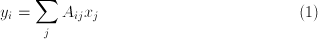
In tomography, the  are cells in space that emit radiation,
and the
are cells in space that emit radiation,
and the  are "bins" of photons collected at particular
angles and locations. In deblurring,
are "bins" of photons collected at particular
angles and locations. In deblurring,  is the original image and
 is the blurry image.
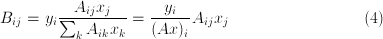
The premise behind Richardson-Lucy is that each contribution from an
element of  to an element of
  has independent Poisson noise:

For the "M" step, we find the most likely value of  based on
 . The most likely value of
  depends on the
  th column
of
th column
of  , which in the absence of noise would be
  times the
corresponding column of
times the
corresponding column of  :
:
For the "E" step, we find the expected value of  given
given
 . The calculation amounts to distributing the value of each
 amongst the
  th row of
  in
proportions according to the known values of
in
proportions according to the known values of  :
:
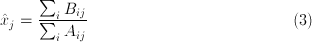
So, here is a way to envision the R-L algorithm at work. Start with a
matrix whose elements are  for some initial guess of
 . Then independently scale each row so that it sums to
  (turning the matrix into an estimate of
  ). Then, replace
each column with a multiple of the corresponding column of
). Then, replace
each column with a multiple of the corresponding column of  having the same sum, and repeat the process. In other words, we
alternate between enforcing two constraints: summing across the rows
of our matrix should yield
having the same sum, and repeat the process. In other words, we
alternate between enforcing two constraints: summing across the rows
of our matrix should yield  , and each column should be a multiple
of the same column in
, and each column should be a multiple
of the same column in  . When the process converges, our matrix
contains valid values of
. When the process converges, our matrix
contains valid values of  .
.
To show that this actually is R-L, we plug  into
into  . We
assume that
. We
assume that  is energy-preserving, so that
  is
is  .
.


In the last equation, for notational convenience, the  represents element-wise multiplication, and the fraction bar
represents element-wise division.
represents element-wise multiplication, and the fraction bar
represents element-wise division.
Ringing: Given the "matrix-update" formulation of R-L given above,
we can see how it is easy for ringing to come about. The ringing
arises in the reconstructed image  , each element of which
corresponds to the scale of a column of the matrix. Basically,
neither update step hinders ringing at all; operating on columns of
the matrix does not relate the
, each element of which
corresponds to the scale of a column of the matrix. Basically,
neither update step hinders ringing at all; operating on columns of
the matrix does not relate the  to each other, and when
operating on the rows, only the sum of each row is considered, which
ignores the oscillation of ringing.
to each other, and when
operating on the rows, only the sum of each row is considered, which
ignores the oscillation of ringing.
Performing basic R-L as described above converges exceedingly slowly and will not match the quality of Matlab's deconvlucy. Matlab uses an acceleration technique which essentially extends each step by a small factor. The Matlab source code references the following papers:
"Acceleration of iterative image restoration algorithms, by D.S.C. Biggs
and M. Andrews, Applied Optics, Vol. 36, No. 8, 1997.

"Deconvolutions of Hubble Space Telescope Images and Spectra",
R.J. Hanisch, R.L. White, and R.L. Gilliland. in "Deconvolution of Images
and Spectra", Ed. P.A. Jansson, 2nd ed., Academic Press, CA, 1997.
The acceleration technique is described in the first paper. Matlab implements the algorithm from sections 2C-D of this paper, and it is not a hard algorithm to implement yourself.