Fast Antialiasing Using Prefiltered Lines on Graphics Hardware

quick links: overview | prefiltering and edge functions | implementation details | downloads and code | references

Introduction Antialiasing for real-time applications is supported in graphics hardware, but its quality is limited by many factors, including a small number of samples per pixel, a narrow filter support, and the use of a simple box filter. See Akenine-Möller and Haines [2002] for a good overview of current hardware antialiasing methods. In this article, I describe a simple method that improves the quality of edge antialiasing by redrawing silhouette edges using prefiltered lines. The technique combines two previous methods, the edge overdraw method of Sander et al. [2001], and the line prefiltering method of McNamara et al. [2000]. I will describe how to implement this combined technique on modern graphics hardware and show quality comparisons with other antialiasing methods. This method has a number of advantages: It support arbitrary symmetric filters at a fixed cost. As we'll see, this is because the lines are prefiltered and the results are stored in small lookup tables. It allows a wider filter support. Most hardware antialiasing schemes only consider samples within a pixel. Unlike the approach of Sander et al. [2001], this method is independent of hardware-specific antialiasing methods. Consequently, results are consistent across platforms. It is a simple, fast, and easy to implement. See the example pixel shader source code below, whose assembly can be hand-optimized to fewer than 10 instructions. The method also has some disadvantages: It requires a polygonal model. It requires explicitly finding discontinuity edges (e.g. silhouettes), which can be expensive for dynamic models. Delay streams, a hardware mechanism recently proposed by Aila et al. [2003], can be used to identify discontinuity edges and reduce the CPU load. It requires an extra rendering pass to draw the discontinuity edges. On the plus side, the number of vertices required is small compared to the entire model. Similarly, the number of pixels drawn at discontinuity edges is a tiny fraction of the framebuffer (typically around 1%). For proper compositing, this method requires a back-to-front sort of the edges. Delay streams can also be used to accelerate this step in hardware. Overview Here is a quick overview of the approach. Draw the scene normally into the framebuffer (without hardware antialiasing). See Figure 1a. Draw wide lines at the objects' silhouettes. Figure 1b shows these lines without the original triangle. These lines can be prefiltered by observing that the convolution of a wide line with a symmetric filter depends only on the distance from the filter to the line. See Figure 1c. (McNamara et al. [2000] show how to handle line endpoints.) In a preprocessing step, we convolve the line with the desired filter at several distances from the line. The resulting intensity values are stored into a small table; see Figure 1d for an example. At run-time, filtering a line only requires a table lookup. Composite the filtered lines into the framebuffer using alpha-blending. See Figure 1e.		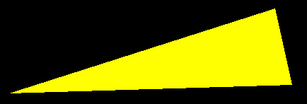Figure 1a. Original aliased geometry. 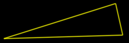Figure 1b. Prefiltered edges. 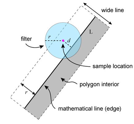Figure 1c. The convolution of a wide line with a symmetric filter can be parametrized by the perpendicular distance d from the sample to the line L. Figure 1d. A 32-entry lookup table indexed by the distance from a sample to the line. This table was computed using a Gaussian filter with std dev 1 pixel. 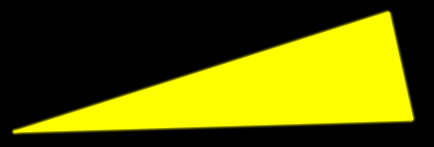Figure 1e. Antialiased result.
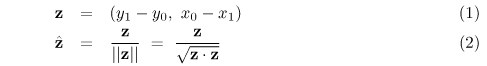
Prefiltering Lines and Edge Functions McNamara et al. [2000] provide the details of computing prefiltered lines using scaled edge functions. I summarize the results and equations in this section. Figure 2 shows the geometric configuration and the relevant variables used in the following equations. Keep in mind that these computations must be performed in window space (i.e., with pixel coordinates). Therefore, transform the object-space endpoints of the line into window space before applying the equations. Consider a line whose endpoints (in pixel coordinates) are (x0, y0) and (x1, y1). 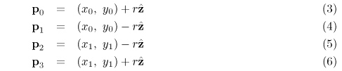First compute the normal to the line: Let r be the filter radius (and also the half-width of the wide line). 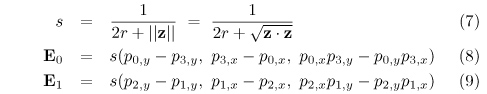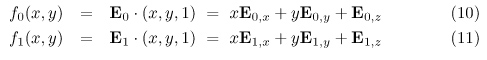Compute the four corners of the wide line: Then compute the linear coefficients of the two (scaled) edge functions: Finally, evaluate the edge functions f for each sample generated by the rasterizer for the wide line: Here, x and y are the pixel coordinates of a given sample. The edge functions in Equations 10 and 11 compute the signed (and scaled) distances from L0 and L1, respectively. In other words, the edge functions produce a value of 1 when the sample is located exactly on L and 0 when the sample is located on the edges of the wide line. If the result of either computation is less than 0, the sample lies outside of the wide line and should be discarded. (This occurs when the rasterizer generates samples that lie slightly outside of the wide line.) For the remaining samples, take the minimum of the functions f0 and f1 and use the result to index into a precomputed one-dimensional lookup table, an example of which is shown in Figure 1d. The result of this lookup is stored into the alpha component of the sample's RGBA color value.		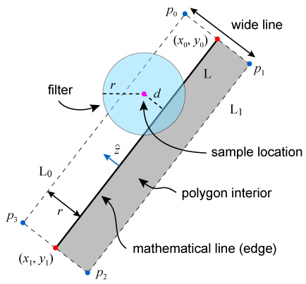Figure 2. Geometric configuration and relevant variables. All calculations are performed using pixel coordinates (i.e., in window space). L is the original (mathematical) line.
Implementation on the GPU In this section, I discuss GPU implementation issues for each step of the algorithm: Draw the scene normally. All texturing, lighting, and other shading calculations should be applied as usual. When drawing the original geometry, it may be necessary to "push back" the geometry slightly in depth to prevent z-fighting with the wide lines. This can be accomplished in OpenGL using glPolygonOffset:     glEnable(GL_POLYGON_OFFSET_FILL);     glPolygonOffset(1.0f, 4.0f); Unfortunately, enabling polygon offset on some GPUs will disable the hardware's early occlusion culling. This is because polygon offset calculations take place during polygon rasterization, whereas early tile-based occlusion culling typically occurs before rasterization begins. Draw wide lines at the objects' silhouettes. Equations 1--9 need to be computed once per line. This can be accomplished on either the host processor or using vertex shaders on the GPU. On the other hand, Equations 10 and 11 must be evaluated for each sample generated by the rasterizer for the wide line. Notice that the scaled edge vectors E0 and E1 from Equations 8 and 9 are designed to make the per-pixel Equations 10 and 11 particularly simple. Discarding unwanted samples is easily accomplished by issuing kill instructions in a fragment program. Textures and Tables I use one-dimensional luminance textures with 32 entries to store lookup tables. An example of such a texture (for a Gaussian) is shown in Figure 1d. I use the hardware-supported box filtering (i.e., GL_LINEAR) when sampling the table, which effectively gives a piecewise-linear approximation to the true intensity falloff curve. Choosing a filter and support size One problem with the antialiasing of commodity graphics hardware is that most of them consider samples only within a single pixel area. In contrast, the approach presented here uses wide lines and thus can take advantage of wider filters. This leaves many questions unanswered, however, such as the choice of filter, support size, and line width. Although we cannot use the ideal sinc filter to eliminate aliasing, we can obtain very good results using a Gaussian truncated at 2 pixels (i.e., a filter with a 2-pixel radius). For example, a sharp edge in 1D filtered using this Gaussian would result in a smooth transition in intensity values across a 4-pixel range. See Figure 3a. There is a problem, however, with applying this method to the lines drawn over the polygon edges. The polygons have already been rasterized into the framebuffer in Step 1 and all color information behind the visible pixels have been discarded. Thus redrawing the edges using prefiltered lines cannot affect the original polygon pixels. In other words, filtering using this approach affects only the pixels that lie outside of the polygon. Consequently, polygons antialiased using this method will appear slightly bloated compared to the original polygons. Naively applying the filter as described above would result in the signal that appears in Figure 3b. This is because the reconstructed signal, in the ideal case, should not achieve its peak value at the edge, but it does so here because of the polygon's pixels residing in the framebuffer. To avoid signal discontinuities, we can adjust the reconstructed signal so that it achieves a peak value at the original edge location, as shown in Figure 3c. This fix, however, can exhibit aliasing, because we have essentially shifted the original edge outwards by one pixel and have applied a filter with a 1-pixel radius. One solution is to shift the edge by 2 pixels and apply a 2-pixel radius filter, as shown in Figure 3d. This greatly reduces the aliasing but noticeably bloats the original geometry. Choosing line width in OpenGL A related issue involves choosing the width of the line to draw. In OpenGL, for example, the line width refers to the number of pixels to draw in each column for x-major lines, i.e. lines with slope in the range [-1, 1]. If we want to ensure that all samples that lie within distance r of a line in screen space are generated by the rasterizer, we need to call glLineWidth with a value of at least ceil(2 * r * sqrt(2)). (Clearly, only samples generated by the rasterizer can be processed in the fragment program.) In practice, for coarse geometry I choose a Gaussian filter (radius r = 2 and std dev 1). For finer geometry, I simply use a box filter with width r = 1. The reason for choosing a narrower filter support is that bloating is more noticeable with finer geometry. I choose the box because using a Gaussian truncated at r = 1 leads to poorer high-frequency rejection and hence more aliasing. Examples of images created using both filters are shown below. Corners One problem with using OpenGL wide lines is that no fragments are generated beyond the endpoints of the line. This makes antialiasing corners of polygons tricky. If we aren't careful about handling the endpoints, we may end up with discontinuities, as shown in Figure 4. This problem naturally gets worse as we choose a larger width r. One solution (although an imperfect one) is to extend the lines slightly in screenspace to form a smoother corner. The examples in Figures 4a and 4b compare results with and without using the line extension. Shading All of the example images presented in this article appear in only a single color (yellow), but the method also applies to shaded objects. All we need are modified versions of the shaders that include the line filtering calculations (e.g., Equations 10 and 11). Composite the filtered lines into the framebuffer using alpha blending. This is accomplished in OpenGL by enabling alpha blending and disabling the depth mask (to prevent the lines from writing depth into the z-buffer):     glEnable(GL_BLEND);     glBlendFunc(GL_SRC_ALPHA, GL_ONE_MINUS_SRC_ALPHA);     glDepthMask(0); Since this blending equation is non-commutative, artifacts may result unless the lines are drawn in back-to-front order (the same is true for transparent polygons). The problem, however, is that correct results are obtained only if sorting is performed in image space for each pixel. Since this cannot currently be done using the z-buffer in conjunction with alpha blending, an approximate sort can be performed in object-space (or equivalently, world-space or eye-space). One heuristic is to use the midpoint of each line to perform sort comparisons [Sander et al. 2001]. Although this heuristic can give incorrect results in some cases, in practice the number of affected pixels is very small. Downloads Click here for a box filter table (TARGA image, 32 entries). Click here for a Gaussian filter table (TARGA image, 32 entries, std dev = 1). Click here for the Cg fragment program for evaluating the edge equations and computing alpha for each line fragment. (Also see code below.) The Cg fragment program for evaluating the edge equations is shown below. void main (out half4 color : COLOR,     float4 wpos : WPOS, // incoming fragment position     uniform float3 E0, // edge equation     uniform float3 E1, // edge equation     uniform sampler1D intensityMap) {     // construct sample position (x, y, 1)     float3 p = float3(wpos.x, wpos.y, 1.0f);     // evaluate edge functions f0, f1     half2 scaledDistance = half2(dot(E0, p), dot(E1, p));     // discard fragments that lie outside the line     if (scaledDistance.x < 0.0f || scaledDistance.y < 0.0f)     {         discard;     }     // choose the relevant distance (edge) to use     half index = min(scaledDistance.x, scaledDistance.y);     // map to alpha using precomputed filter table     half alpha = tex1D(intensityMap, index);     //     // do other shading here ...     //     // color.xyz = ...     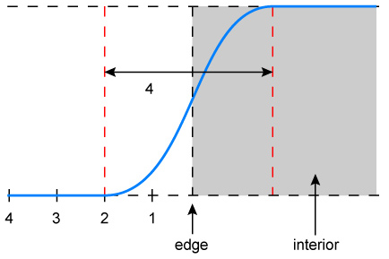color.w = alpha; }		Figure 3a. Bandlimited signal obtained by filtering a sharp edge with a Gaussian with radius 2. 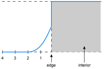Figure 3b. The signal of the original polygon is written into the framebuffer and cannot be modified. Applying the prefiltered lines directly at the edge leads to this discontinuity. 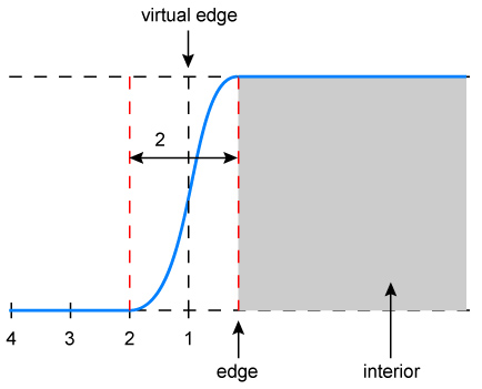Figure 3c. The prefiltered line can be adjusted to attain its peak value at the original edge. This is equivalent to convolving the indicated virtual edge with a filter of radius 1. However, using this narrower filter increases aliasing. 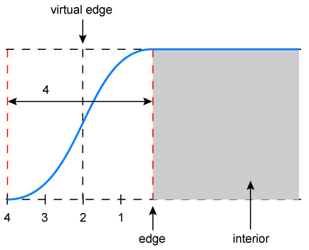Figure 3d. Better results are obtained by shifting the virtual edge outwards by an additional pixel and using a filter of radius 2. Unfortunately, this gives the geometry a somewhat "bloated" appearance. 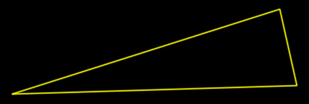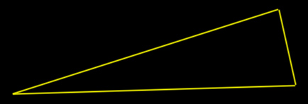Figure 4a. Box filter, r = 1, with and without line extension. 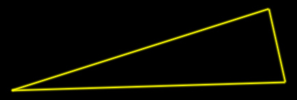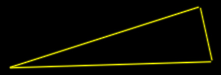Figure 4b.. Gaussian filter (std dev = 1), r = 2, with and without line extension.
Examples and Comparisons This section uses images of a single yellow triangle to compare prefiltered edge overdraw with existing hardware antialiasing methods. The first set of images shows the entire triangle at 100% magnification. The differences in quality are apparent in the still images and even more so in animations. Figure 5a. Original scene, no antialiasing. Figure 5b. NVIDIA Quadro FX 2000, 16x AA (4x4 ordered grid).   Figure 5c. ATI Radeon 9800 Pro, 6x (rotated grid, interleaved). Figure 5d. Sander et al. [2001] (hardware line antialiasing).   Figure 5e. Prefiltered, box (r = 1). 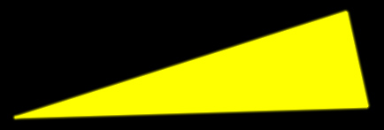Figure 5f. Prefiltered, Gaussian (std dev = 1, r = 2). Closeup #1 The next set of images show a closeup of one of the triangle's nearly horizontal edges. 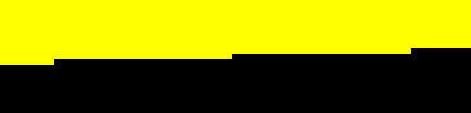Figure 6a. Original scene, no antialiasing. 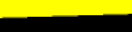Figure 6b. NVIDIA Quadro FX 2000, 16x AA (4x4 ordered grid).  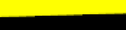 Figure 6c. ATI Radeon 9800 Pro, 6x (rotated grid, interleaved). 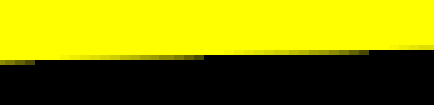Figure 6d. Sander et al. [2001] (hardware line antialiasing).  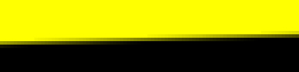 Figure 6e. Prefiltered, box (r = 1). 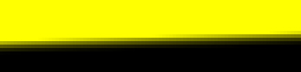Figure 6f. Prefiltered, Gaussian (std dev = 1, r = 2). Closeup #2 The next set of images show a closeup of one of the triangle's other edges and includes a sharp corner. I used line extension for the prefiltered edges to reduce artifacts at the corner. 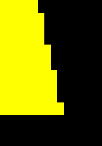Figure 7a. Original scene, no antialiasing.  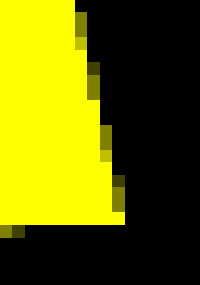 Figure 7b. NVIDIA Quadro FX 2000, 16x AA (4x4 ordered grid).  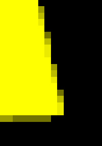 Figure 7c. ATI Radeon 9800 Pro, 6x (rotated grid, interleaved).   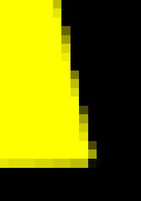Figure 7d. Sander et al. [2001] (hardware line antialiasing).  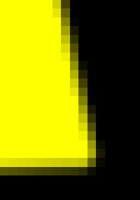 Figure 7e. Prefiltered, box (r = 1).  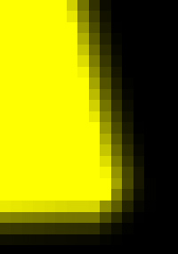 Figure 7f. Prefiltered, Gaussian (std dev = 1, r = 2).
Conclusions This article has described a method for implementing prefiltered line antialiasing on the GPU. Combining this approach with the discontinuity edge overdraw algorithm leads to polygon edges of much higher quality. The key limitations of this approach -- the need to find discontinuity edges explicitly and the need to draw edges back-to-front -- can be overcome with additional hardware, such as a delay stream.
References Timo Aila, Ville Miettinen, and Petri Nordlund. Delay Streams for Graphics Hardware. Proceedings of ACM SIGGRAPH. ACM Press, 2003. More info. Tomas Akenine-Möller and Eric Haines. Real-Time Rendering, 2nd ed. A.K. Peters, Ltd., 2002. More info. Robert McNamara, Joel McCormack, and Norman P. Jouppi. Prefiltered Antialiased Lines Using Half-Plane Distance Functions. Proceedings of the ACM SIGGRAPH/EUROGRAPHICS Workshop on Graphics Hardware. ACM Press, 2000. More info. Pedro V. Sander, Hugues Hoppe, John Snyder, and Steven J. Gortler. Discontinuity Edge Overdraw. Proceedings of the 2001 Symposium on Interactive 3D Graphics. ACM Press, 2001. More info.