Two bag-of-words classifiers
ICCV 2005 short courses on
Recognizing and Learning Object Categories
|
|
Two bag-of-words classifiers ICCV 2005 short courses on Recognizing and Learning Object Categories |
|
A simple approach to classifying images is to treat them
as a collection of regions, describing only their appearance and
igorning their spatial structure. Similar models have been
successfully used in the text community for analyzing
documents and are known as "bag-of-words" models, since each
document is represented by a distribution over fixed
vocabulary(s). Using such a representation, methods such as probabalistic latent semantic
analysis (pLSA) [1] and latent dirichlet allocation (LDA) [2] are able to extract coherent topics
within document collections in an unsupervised
manner.
Recently, Fei-Fei et al. [3] and Sivic et al. [4] have applied such methods to the visual domain. The demo code implements pLSA, including all pre-processing stages. For comparison, a Naive Bayes classifier is also provided which requires labelled training data, unlike pLSA. The code consists of Matlab scripts (which should run under both Windows and Linux) and a couple of 32-bit Linux binaries for doing feature detection and representation. Hence the whole system will need to be run on Linux. The code is for teaching/research purposes only. If you find a bug, please email me at fergus where csail point mit point edu. |
|
Download Download the code and datasets (32 MBytes): tgz file zip file Operation of code To run the demos: 1. Unpack the .zip file into a new directory (e.g. /home/username/demos) 2. Put the common/ directory in your Matlab path (by doing 'addpath /home/username/demos/common'). This directory holds all the code used in the experiments 3. move into one of the experiment directories, e.g. 'cd /home/username/demos/experiments/parts_structure' 4. ensure that the paths at the top of the config_file_1.m file are correct. (i.e. swap 'fergus' for 'username' or whatever). 5. Then you are good to go. Type 'doall('config_file_1')' and it all run. Since the training is manual, you will need to do some clicking at some point, but the rest is automated. For an overview of what is going on see the sections below. For a more detailed understanding, read the comments in the .m files. Description of code Experiment script config_file_1.m - Each experiment has its own script. This holds ALL settings required to reproduce the experiment in its entirety. The script should sit in its own subdirectory within experiments/. Each of the 'do_' functions is passed the script. The parameters and settings are grouped into structures for neatness. At the top of the script, the paths to various key directories are set. Before running ensure that these are correct. At the very top of the script is the EXPERIMENT_TYPE variable, used by do_all.m to call the appropriate sub-stages. For these demos, it should either be 'plsa' or 'naive_bayes'. Top-level function do_all.m - Master function that calls all the different section of the algorithms in turn. The choice of the algorithm is made by the EXPERIMENT_TYPE setting in the configuration file. Stages of the algorithm do_random_indices.m - randomly picks the training and test indices as stores them in a file in the current experiment directory. do_preprocessing.m - copies and rescales (as specified) all images from the IMAGES_DIR into the images/ directory in the current experiement directory. do_interest_op.m - Runs a very crude interest operator over the images to gather a set of regions. See Edge_Sampling.m for details of the operator. A Caddy edge detector is used, which is implemented as binary (both Windows and Linux versions are provided). do_representation.m - takes the regions produced by do_interest_op.m and characterises their appearance, in this instance using SIFT features. This is done by means of a linux binary. do_form_codebook.m - Runs k-means on the SIFT vectors from all training images to build a visual vocabulary. Uses a Linux .mex file, but source code is provided so you can recompile for any platform you wish. do_vq.m - Vector quantizes the regions from all images using the vocabulary built by do_form_codebook.m. do_plsa.m - Learns a pLSA model from the training images. The number of topics is specified in Learn.Num_Topics in the configuration file. do_plsa_evaluation.m - Test a pLSA model on the testing images. Plots ROC and RPC curves as well as test images with regions overlaid, colored according to their preffered topic. do_naive_bayes.m - Forms a Naive Bayes classifier from the training images. do_naive_bayes_evaluation.m - Tests the Naive Bayes classifier on the testing images. Plots ROC and RPC curves as well as test images with regions overlaid, colored according to their preffered topic. |
|
Walkthough of demo Sample images This is a sample of the images used for this demo. It contains a mix of faces from the Caltech face dataset and images from the Caltech background datasets. The do_preprocessing.m script should resize all of them to 200 pixels in width. 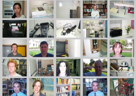
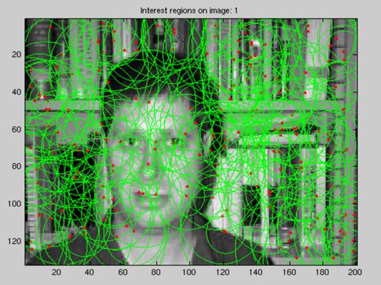
Interset point operator Running do_interest_op.m calls the crude interest operator, Edge_Sampling.m. This runs a Canny Edge detector over the image and then samples points from the set of edgels. The scale is also determined by randomly sampling over a uniform distribution. The two images below show the set of edgels and sampled regions for a typical image. 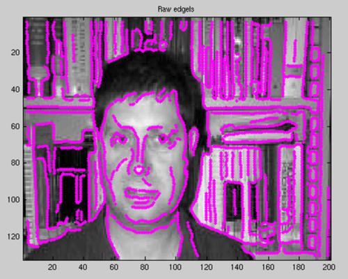
Representation Running do_representation.m produces SIFT vectors for each interest point. Once a visual vocabulary or codebook has been built and the do_vq.m procedure has been run, each interest point file should contain the variables shown in the figure below (in this image, there are 154 regions - this number will vary from image to image): 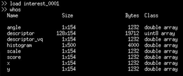
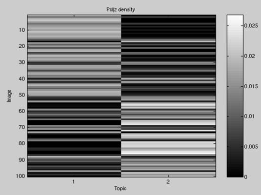
Training Running do_plsa.m should produce output like (n.b. it will not be identical due to the random initialization of the model): >> do_plsa('config_file_1') Iteration 1 dLi=0.000000 Iteration 2 dLi=225.753173 Iteration 3 dLi=142.124978 Iteration 4 dLi=114.276770 Iteration 5 dLi=102.580805 Iteration 6 dLi=95.619991 Iteration 7 dLi=89.379039 Iteration 8 dLi=83.222576 Iteration 9 dLi=78.063911 Iteration 10 dLi=74.565845 Iteration 11 dLi=72.679587 Iteration 12 dLi=72.276609 Iteration 13 dLi=73.070117 Iteration 14 dLi=74.539317 ... It should finish after 100 iterations. Evaluation Running do_plsa_evaluation.m will then produce (after a few more EM iterations) several figures. Below are plots of the p(w|z) (on left) and p(d|z) (on right) densities: 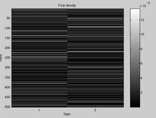
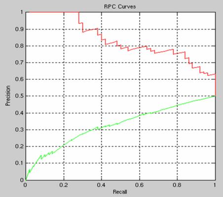
Then the ROC and RPC curves are shown for classification task (face present/absent) only - the bag of words models cannot localize. 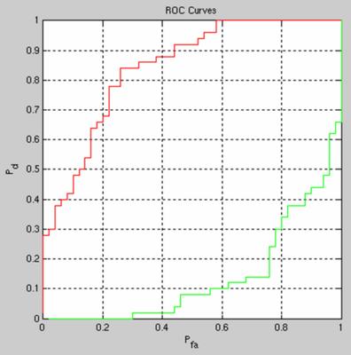
 Finally, some example images are plotted with the regions overlaid, coloured according to their preferred topic: 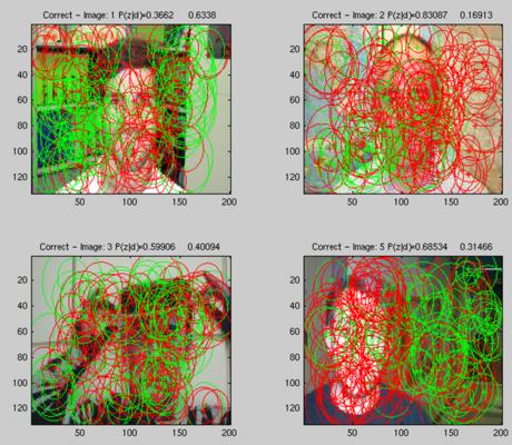
References [1] Hofmann, T., "Probabalistic Latent Semantic Analysis", UAI 1999. [2] Blei, D. and Jordan, M., "Latent Dirichlet Allocation",Journal of Machine Learning Research, 3:993-1022, January 2003. [3] Fei-Fei, L. and Perona, P., "A Bayesian Heirarcical Model for Learning Natural Scene Categories", Proc. CVPR, 2005. [4] Sivic, J. and Russell, B. and Efros, A. and Zisserman, A. and Freeman, W., "Discovering object categories in image collections." Proc. Int'l Conf. Computer Vision, Beijing, 2005. |