A simple parts and structure object detector
ICCV 2005 short courses on
Recognizing and Learning Object Categories
|
|
A simple parts and structure object detector ICCV 2005 short courses on Recognizing and Learning Object Categories |
|
An intuitive way to represent objects is as a collection of
distinctive parts. Such schemes model both the relative
positions of the parts as well as their appearance, giving a
sparse representation that captures the essence of the object.
This simple demo illustrates the concepts behind many such "parts and structure" approaches. For simplicity, training is manually guided with the user hand-clicking on the distinctive parts of a few training images. A simple model is then built for use in recognition. Two different recognition approaches are provided: one relying on feature points [1]; the other using the efficient methods of Felzenswalb and Huttenlocher [2]. The code consists of Matlab scripts (which should run under both Windows and Linux). The Image Processing toolbox is required. The code is for teaching/research purposes only. If you find a bug, please email me at fergus where csail point mit point edu. |
|
Download Download the code and datasets (24 MBytes): tgz file zip file Operation of code To run the demos: 1. Unpack the .zip file into a new directory (e.g. /home/username/demos) 2. Put the common/ directory in your Matlab path (by doing 'addpath /home/username/demos/common'). This directory holds all the code used in the experiments 3. move into one of the experiment directories, e.g. 'cd /home/username/demos/experiments/parts_structure' 4. ensure that the paths at the top of the config_file_1.m file are correct. (i.e. swap 'fergus' for 'username' or whatever). 5. Then you are good to go. Type 'doall('config_file_1')' and it all run. Since the training is manual, you will need to do some clicking at some point, but the rest is automated. For an overview of what is going on see the sections below. For a more detailed understanding, read the comments in the .m files. Description of code Experiment script config_file_1.m - Each experiment has its own script. This holds ALL settings required to reproduce the experiment in its entirety. The script should sit in its own subdirectory within experiments/. Each of the 'do_' functions is passed the script. The parameters and settings are grouped into structures for neatness. At the top of the script, the paths to various key directories are set. Before running ensure that these are correct. At the very top of the script is the EXPERIMENT_TYPE variable, used by do_all.m to call the appropriate sub-stages. For these demos, it should either be 'parts_structure' or 'parts_structure_efficient'. Top-level function do_all.m - Master function that calls all the different section of the algorithms in turn. The choice of the algorithm is made by the EXPERIMENT_TYPE setting in the configuration file. Stages of the algorithm do_random_indices.m - randomly picks the training and test indices as stores them in a file in the current experiment directory. do_preprocessing.m - copies and rescales (as specified) all images from the IMAGES_DIR into the images/ directory in the current experiement directory. do_manual_train_parts_structure.m - presents the training set to the user, for he/she to select distinctive parts of the object. Once all training images have been clicked by the user, a simple parts and structure model is built and saved in the models/ subdirectory, along with a copy of the configuration_script. do_part_filtering.m - takes the filters created by the manual clicking and uses them as matched filters on the training and test images. For each image, normalised cross-correlation is used to give the response of the filter over the whole image. Local maxima of this "response image" are taken, giving a set of interest points. do_test_parts_structure.m - evaluates the model using the interest points identified. do_test_efficient.m - evaluates the model using the efficient methods of Felzenswalb and Huttenlocher. |
|
Walkthough of demo Sample images This is a sample of the images used for this demo. It contains a mix of faces from the Caltech face dataset and images from the Caltech background datasets. The do_preprocessing.m script should resize all of them to 200 pixels in width. 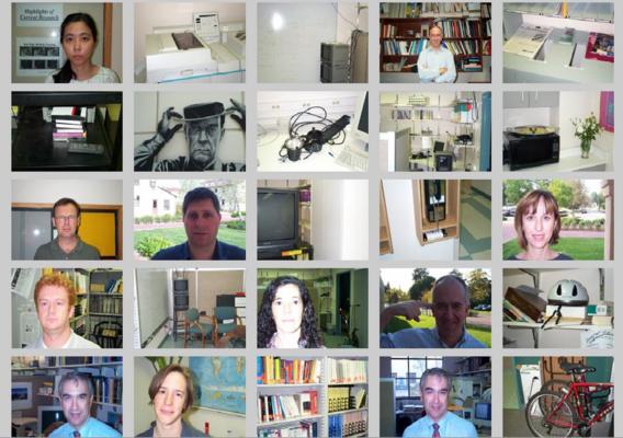
Manual Training The manual training consists of clicking on point on the faces. A red dot indicates the location of the click, while a red rectangle shows the scale of the region taken from the image. The figure below illustrates this procedure: 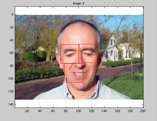
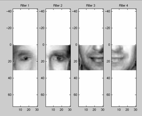
Once all training images have been manually annotated, the shape model (relative to the 1st part) and filters (pixel averages of regions selected for each part) are shown. These form the shape and appearance models for use in recognition. 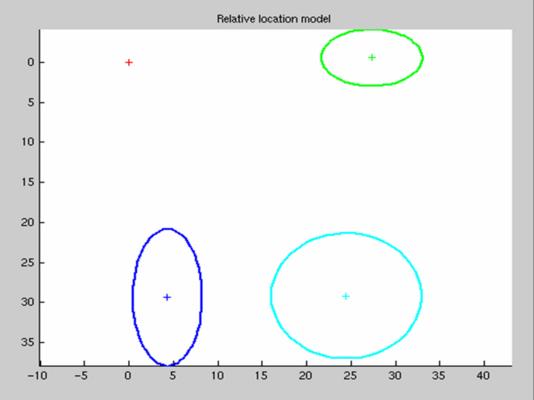
Filtering The filters computed in training are now applied to the images using normalized cross-correlation. The figures below show the response maps for each model part on a single image, with the black dots indicating local maxima which are taken as interest points in recognition. 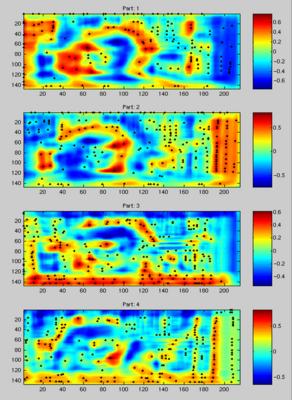
The interest points extracted for each part on the image are shown below (coloured according to their part). 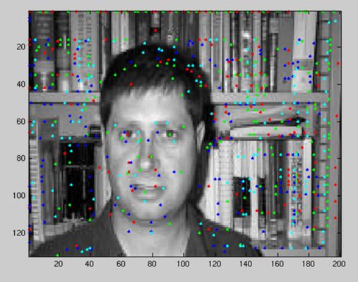
Recognition The spatial model is now applied to the interest points and the best combination found over each image. The score for each match is a weighted combination of the probabilty under the shape model and the normalized correlation response over at the interest points for each part. The ROC curve below (left) evaluates classification performance (face present/absent) and the RPC curve below (right) shows the localization performance. 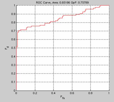 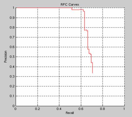
The examples in the image below show the best match with coloured crosses; the proposed bounding box (a constant scale factor larger than the bounding box of the best match) in green or red depending if it was correct or not; the ground truth bounding box in blue. The interest points for each parts are also plotted. 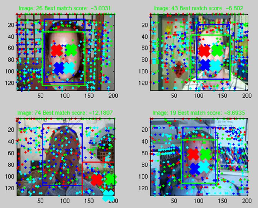 References [1] Fischler, M. and Elschlager, R. "The representation and matching of pictorial structures." IEEE Transactions on Computers, 22(1):67--92, 1973. [2] Felzenszwalb, P. and Huttenlocher, D. "Pictorial Structures for Object Recognition." Intl. Journal of Computer Vision, 61(1), pp. 55-79, January 2005. |