 Paper
(PDF)
Paper
(PDF) Check out our new paper for a fast bilateral filter with better accuracy and formal analysis. Code is available. The web page also has links to various utilizations of the bilateral filter and relevant work.
If you are struggling to implement our tone mapping algorithm, see notes at the end of the page. I noticed that people's implementation often don't match mine.
The choices we make (talk at Harvard where I discuss the many levels of choice involved in this project and which ones I deem important vs. incidental) (ppt, pdf)
Abstract:
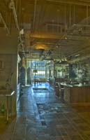
We present a new technique for the display of high-dynamic-range-images, which
reduces the contrast while preserving detail. It is based on a two-scale decomposition
of the image into a base layer, encoding large-scale variations, and a detail
layer. Only the base layer has its contrast reduced, thereby preserving detail.
The base layer is obtained using an edge-preserving filter called the bilateral
filter. This is a non-linear filter, where the weight of each pixel is computed
using a Gaussian in the spatial domain multiplied by an influence function in
the intensity domain that decreases the weight of pixels with large intensity
differences. We express bilateral filtering in the framework of robust statistics
and show how it relates to anisotropic diffusion. We then accelerate bilateral
filtering by using a piecewise-linear approximation in the intensity domain
and appropriate subsampling. This results in a speedup of two orders of magnitude.
The method is fast and requires no parameter setting.

 Slides
(PPT, PDF 1 per
page or 6
per page)
Slides
(PPT, PDF 1 per
page or 6
per page)
Fast Forward slides (2 slides only) PPT
More background on contrast management and the limitations of the medium in our SIGGRAPH course Perceptual and Artistic Principles for Effective Computer Depiction
Note that we have filed a US patent application for the technique.
In Greg Ward's Radiance format. Images courtesy of Byong Mok Oh, acquired using multiple-exposure photography with a Nikon D1 digital camera, and combined using the HDRShop software.
 |
 |
Kate Devlin. A review of tone reproduction techniques
Ward-Larson et al., A Visibility Matching Tone Reproduction Operator for High Dynamic Range Scenes
J. DiCarlo and B. Wandell, Rendering High Dynamic Range Images
Reinhard et al., Photographic
Tone Reproduction for Digital Images
Fattal et al. Gradient Domain High Dynamic Range Compression
Ashikhmin A Tone Mapping Algorithm for High Contrast Images
Jobson et al. Multiscale Retinex
Socolinsky, Dynamic Range Constraints in Image Fusion and Visualization
Pattanaik et al. A Multiscale Model of Adaptation and Spatial Vision for Realistic Image Display
S. N. Pattanaik, Hector Yee, Adaptive Gain Control for High Dynamic Range Image Display
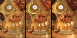
Many people have asked for a comparison between the three papers published at SIGGRAPH this year
First, we have informal comparison slides. I insist. The comparison is informal, and it is hard to draw conclusions from only two different inputs. Moreover, the various authors use different reduction strategies, which can be (by choice) more or less aggressive in terms of contrast reduction. We also realized that we used different gamma correction. We tried to manually correct this, but it is only a had-oc fix. Basically most paper focus on contrast reduction for the intensity only.
My initial informal impressions are as follows:
First of all, all three techniques perform very well. The gradient domain technique seems to be the best at preserving detail, maybe sometimes too good. Our bilateral technique is the fastest, but this could be due to more careful optimization. It might provide a more photographic look that the gradient domain method, because highlights are more saturated, which results in a less flat picture. However, the blacks are not as deep. I am investigating where this is coming from. The photographic technique is, not surprisingly, the one that best provides a photographic appearance. It actually consists in two complementary methods, a global one and a local one. The global method is by far the simplest technique of all recent tone-mapping operators, and it is lightning fast. The local method share similarities with both Ashikhmin's and our work, in that it blurs but avoids blurring across edges. Which incidentally means that the bilateral filter could be used instead. In my opinion, the bilateral filter provides a better estimate because it has a larger spatial support: the other two methods basically use an increasing blurring radius, and stop as soon as an edge is encountered, while the bilateral filter will "use" all valid pixel in a given radius.
A note related to Ashikhmin's paper. The output of the bilateral filter can be used as the adaptation value for most global tone mapping methods. Indeed, in my implementation, the base layer is called "adaptation". I have used Ward's 94 technique, Ferwerda's 96 technique and Tumblin's brightness-based method with equal success. We all agree that the adaptation computed using the bilateral filter is not strictly speaking the adaptation value that drives the human visual receptors, but this does a good job at approximating what's going on in the eye.
Tomasi and Manducci's original paper
Greg Ward's PhotoPhile browser
A site about contrast sensitivity
In Fig. 10 (pseudocode), minI and min(I) are the same thing.
InterpolationWeight is simply the linear interpolation basis function. That is, it is a triangle-shaped function that is defined as
InterpolationWeight(x)=
Here is the high-level set of operation that you need to do in order to perform contrast reduction
input intensity= 1/61*(R*20+G*40+B)
r=R/(input intensity), g=G/input intensity, B=B/input intensity
log(base)=Bilateral(log(input intensity))
log(detail)=log(input intensity)-log(base)
log (output intensity)=log(base)*compressionfactor+log(detail) - log_absolute_scale
R output = r*10^(log(output intensity)), etc.
You can replace the first formula by your favorite intensity expression.
You can replace the multiplication by compressionfactor by your favorite contrast-reduction curve (e.g. histogram adjustment, Reinhard et al.'s saturation function, etc.)
The memorial church result might have undergone a questionable gamma transform before our algorithm was applied. This might explain discrepancies with other implementation of our technique.
compressionfactor and log_absolute_scale are image-dependent. compressionfactor
makes sure the contrast matches a given target contrast. It is the ratio of
this target and the contrast in the base layer:
targetContrast/(max(log(base)) - min(log(base)))
I use log(5) as my target, but you can use a bigger value to preserve more contrast.
log_absolute_scale essentially normalizes the image, by making sure that the biggest value in the base after compression is 1. It is equal to max(log(base))*compressionfactor
All log are in base 10.