Capturing Linear Images
01 July 2009
In a recent project, I had to capture and process linear images. In a linear image, the value at every pixel is directly related to the number of photons received at that location on the sensor. While most people do not have to worry about linearity, and in fact, consumer cameras apply nonlinear response curves to the captured data, scientists often derive relationships that assume linearity. In this post, I describe several methods for achieving linear images and describe a few pitfalls that I encountered while attempting to capture linear images.
Most semi-professional and professional cameras allow the images to be stored in a RAW format. This format encodes the sensor data before the in-camera processing that is used to produce more familiar image formats, such as JPEG. The RAW format has been called the digital equivalent of the negative and the format allows a user to adjust parameters to produce a final image in the same way that professional photographers would adjust their images using darkroom techniques.
The RAW format is a linear image, but it is not the easiest format to work with since it is specific to a camera manufacturer. In order to analyze RAW images in mathematical software such as MATLAB, you must convert them to a more common format. But depending on how you do the conversion, you may end up with images that are not linear. For those who need linearity, I have documented several workflows that preserve it. I also describe my methodology for checking linearity.
Data capture
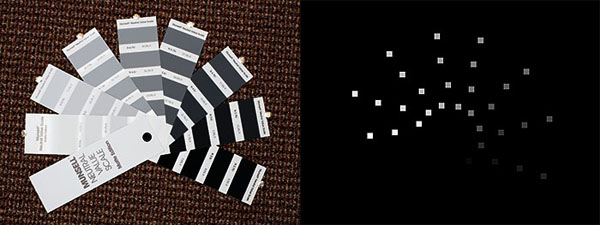
For all tests, I used a Munsell Neutral Value Scale, matte edition. The scale is
a fan deck with 31 patches of various shades of gray, shown on the left below.
Note that I am assuming that the lighting across the scale is uniform and that
the individual cards in the scale are lying flat. To analyze images of the
scale, I made a mask in Photoshop to sample a 64 x 64 section of each patch. The mask is shown on the right below.
The Munsell scale has a reflectance percentage printed below each of the 31 patches. These values are:
| Patch | Reflectance | Patch | Reflectance | Patch | Reflectance |
|---|---|---|---|---|---|
| 1 | 3.1 | 12 | 17.6 | 23 | 50.7 |
| 2 | 3.8 | 13 | 19.8 | 24 | 54.8 |
| 3 | 4.6 | 14 | 22.1 | 25 | 59.1 |
| 4 | 5.5 | 15 | 24.6 | 26 | 63.6 |
| 5 | 6.6 | 16 | 27.2 | 27 | 68.4 |
| 6 | 7.7 | 17 | 30.0 | 28 | 73.4 |
| 7 | 9.0 | 18 | 33.0 | 29 | 78.7 |
| 8 | 10.4 | 19 | 36.2 | 30 | 84.2 |
| 9 | 12.0 | 20 | 39.5 | 31 | 90.0 |
| 10 | 13.7 | 21 | 43.1 | ||
| 11 | 15.6 | 22 | 46.8 |
I created the mask so that it would be simple to map the intensity value in the mask to the reflectance value printed on the Munsell scale: the value of each patch was 8 times the patch index. Therefore, I could divide the value in the mask by 8 and use the result as an index into the reflectance table above. Note that I configured Photoshop to use a linear colorspace when making the mask so that the numerical values in the PNG file (as read in MATLAB) would be the same values I specified in Photoshop (and not gamma-mapped in any way). The tutorial I used to create a linear colorspace can be found here.
Photoshop Camera RAW
Photoshop is able to load and process RAW images using the Camera RAW plugin released in 2003. I loaded my RAW image (a Nikon NEF file) and saved it as a 16-bit PNG. I then loaded the image in MATLAB plotted the intensities at the patches in the mask versus the known reflectances. The plot below shows that the data stored in the PNG file is not linear, even though I used a linear tone curve in the Camera RAW dialog and set all sliders in the Basic panel to 0. The black dashed lines show the best linear fit to the data in each channel.
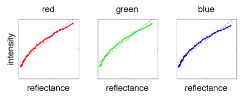
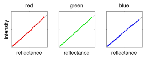
The problem was that the colorspace was set to sRGB in the Camera RAW workflow (accessed by clicking the link at the bottom of the Camera RAW dialog). One option is to change the image to 32 bits (Image->Mode->32 Bits/Channel) and save as a 32-bit file type, such as OpenEXR. Another option is to convert the image to a linear colorspace (Edit->Convert to Profile…), created according to the instructions mentioned above, and then save the image as a PNG. When the settings are correct, the plot of intensities versus reflectances should be close to linear, as shown below.
dcraw
For those who do not own Photoshop, there is a free conversion utility known as dcraw. I was able to convert the RAW file to a linear image using the following options:
dcraw -v -4 -H 0 -W -w -q 3 file.nef
where file.nef is a Nikon RAW file. I also checked that these options would yield linear images for Canon CRW files. The definitions of the options can be found in the dcraw documentation, or in related tutorials, such as this tutorial.
Photoshop Merge to HDR
One final method for capturing linear images is to photograph the scene at several different exposures and merge the images into a high dynamic range (HDR) image using Photoshop. This option is also useful if the scene luminance exceeds the dynamic range of your camera (both dark blacks and bright highlights).
In Photoshop, the Merge to HDR option is available under File->Automate and you select several files to be merged into a single image. I found that the 32-bit HDR image could be saved as a 32-bit image and the resulting image was linear when loaded in MATLAB.
Conclusions
If linearity is important to your project, I suggest verifying the linearity of your entire workflow using the approach I described here. With several different tools and file formats in the workflow, it is possible a gamma is being applied at some point without you realizing it. For example in Photoshop, a pitfall to be aware of is how colorspace settings can affect common image operations. In the default colorspace, I found that operations such as grayscale conversion (Image->Mode->Grayscale) and copy-paste (without explicitly setting the colorspace) would affect the linearity of the image. For these reasons, I suggest testing your entire workflow for linearity.