
The complete formula is the following, and the variables are explained below:
Theta = heading direction
V
= Speed
B
= Damping
K, G1, G2 = Goal parameters
E1, E2, O1, O2 = Obstacle parameters
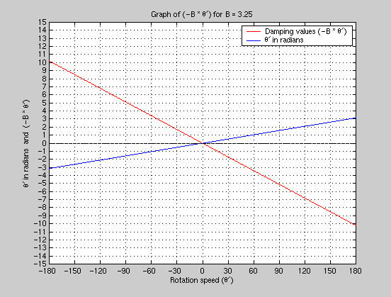
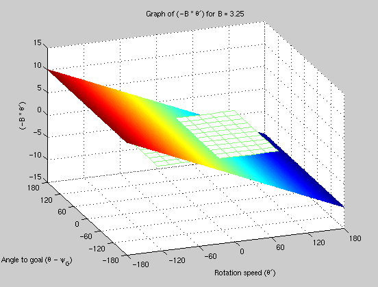
The followings are example graphs demonstrating the contribution of the damping part to the computation of rotation acceleration with B = 3.25
 |
 |
|
|
Damping values are plotted against the "angle to goal" (goal direction with respect to the agent's heading) values. Zero plane is also shown explicitly in green. |
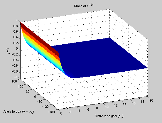
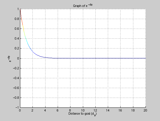
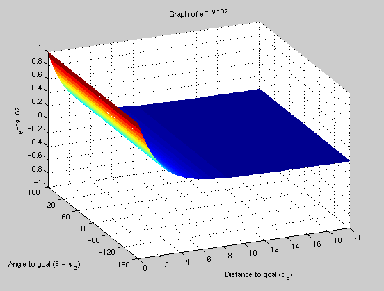
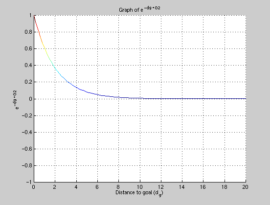
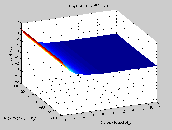
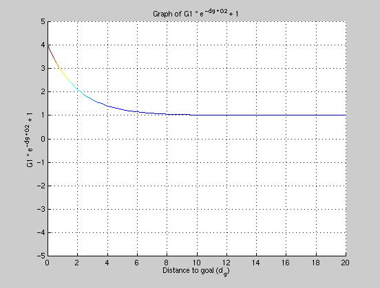
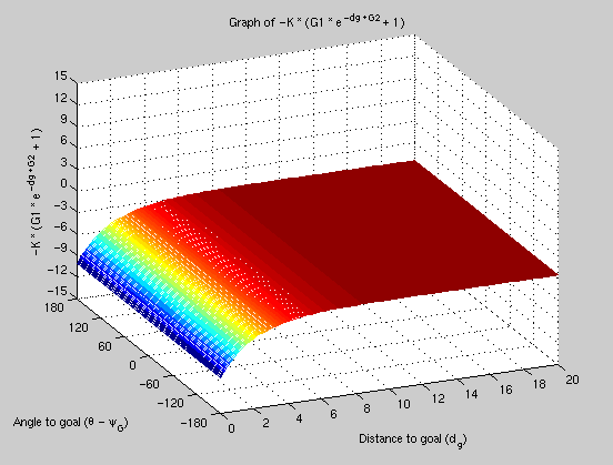
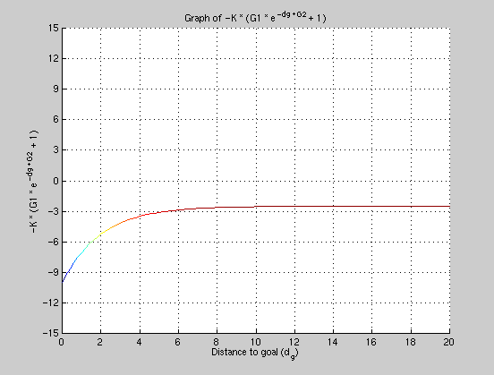
The following graphs are plotted using these example values:
 |
 |
 |
 |
 |
 |
 |
 |
|
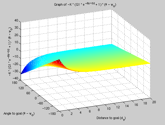
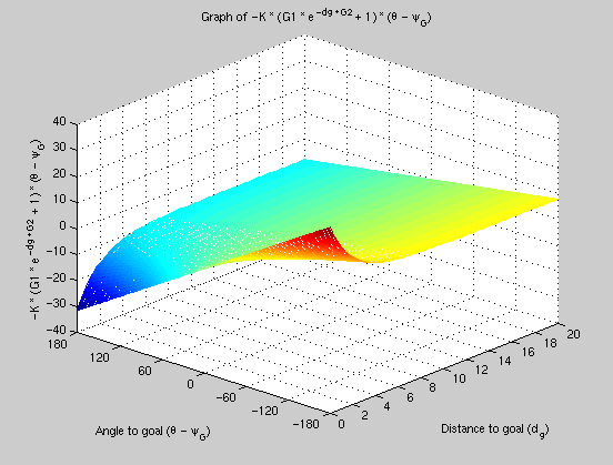
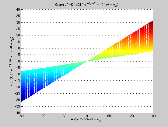
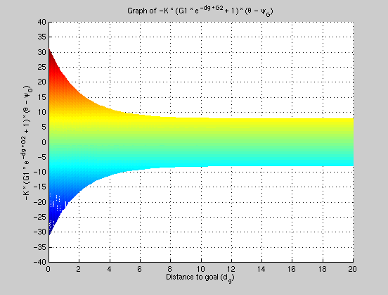
Until now, we prepared the "decreasing influence" of the goal, now we'll also include the effect of goal direction. Below are 4 different views of the resulting graph: |
|
 |
 |
 |
 |
|
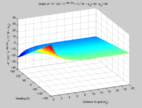
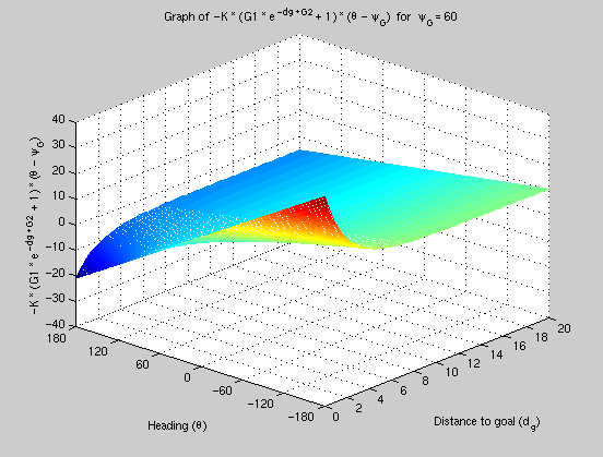
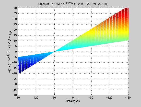
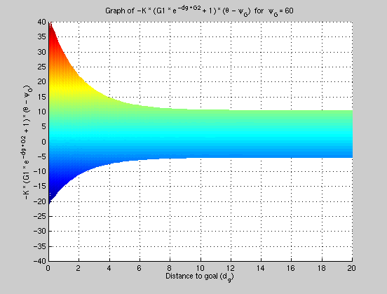
To see the effect of heading on the target part, let's plot the target contribution against heading (with psi_G = 60 degrees) instead of the net angle to goal. The result is simply a shift (equal to psi_G) of the graph values. Below are 4 views of the resulting graph (with the same corresponding view angles as above graphs): |
|
 |
 |
 |
 |
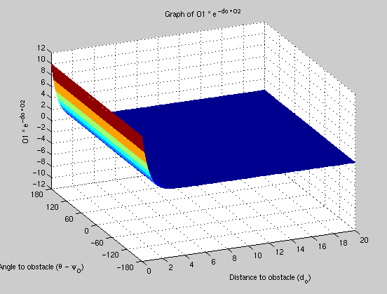
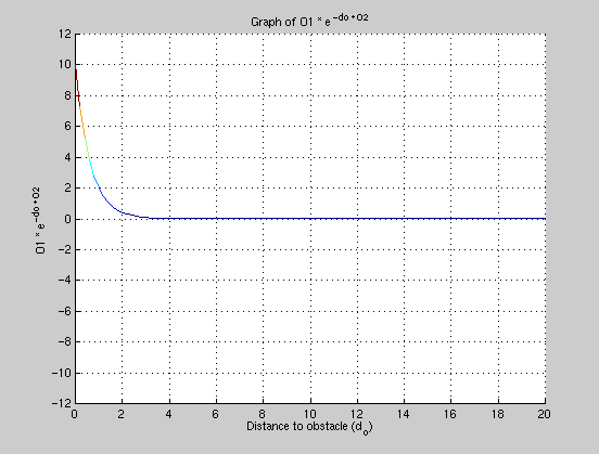
The following values are used while drawing the graphs:
 |
 |
 |
 |
 |
 |
|
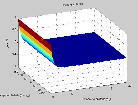
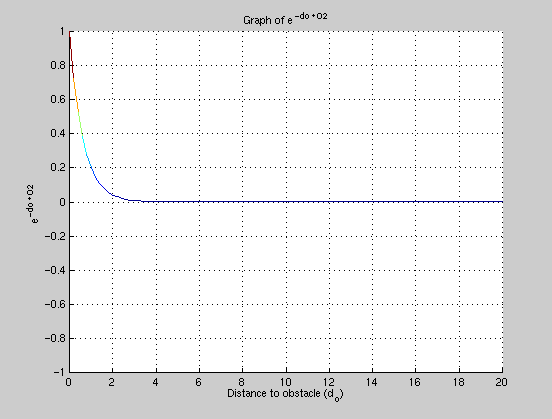
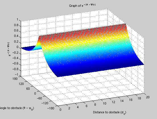
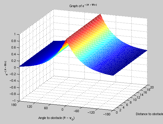
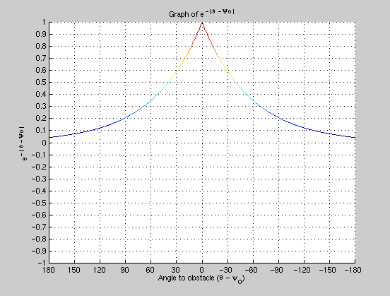
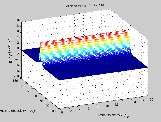
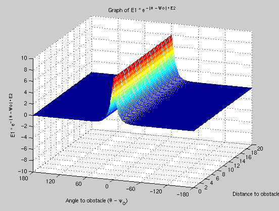
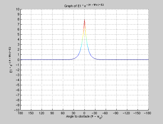
The first section of the formula which deals with the effect of distance is ready. The second section dealing with the magnitude of the "angle to obstacle" is constructed below: |
|
|
|
 |
 |
 |
|
|
 |
 |
 |
|
|
 |
 |
 |
|
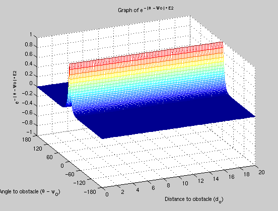
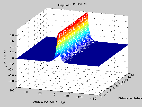
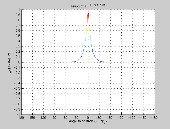
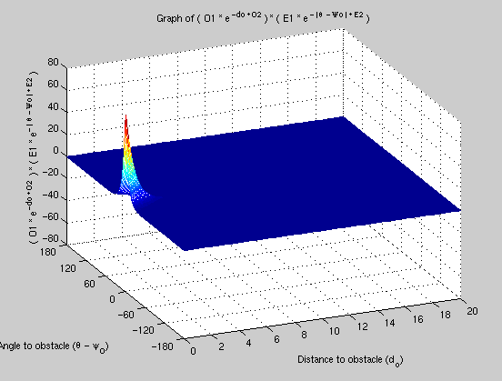
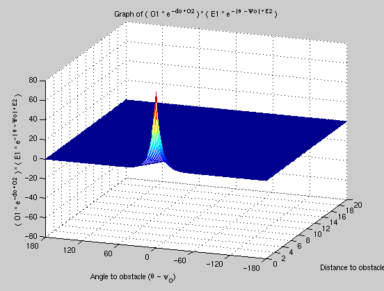
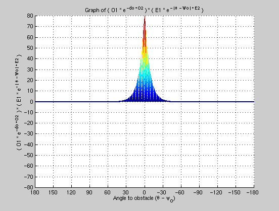
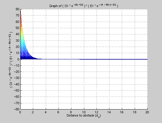
Now we combine the "magnitude of the angle" influence and the distance influence to get the following graph (shown in 4 different views): |
|
 |
 |
 |
 |
|
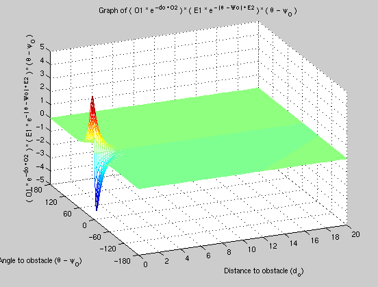
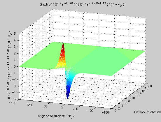
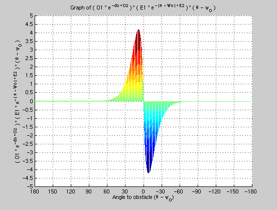
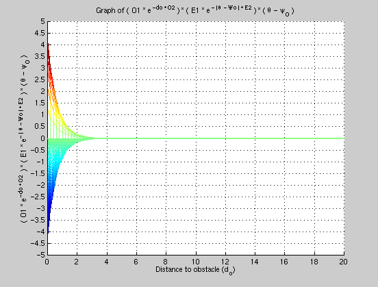
Last step is to include the obstacle direction influence. Below is the final graph showing the effect of a single obstacle (in 4 different views): |
|
 |
 |
 |
 |