Optical Flow Based Robot Navigation
Abstract
Our aim is to develop algorithms that will be used for
robust visual navigation of mobile autonomous agents. The approach is to
efficiently compute and use optical flow fields to extract the features
of the environment that are important for our purpose and to use this information
as our guide for motion. We are using image frames supplied by both a monocular
vision system of a physical robot and a simulated environment as the input
for testing our algorithms. The raw images from these continuous image
sequences are first converted to SLOG images, and then a patch
matching is applied to these preprocessed images to obtain the optical
flow field. Currently, two programs that we have designed make use of the
computed flow information to avoid obstacles by a method called the balance
strategy, and to estimate the time to contact with a surface.
Contents
Optical Flow Algorithm
In an image, each pixel corresponds to the intensity
value obtained by the projection of an object in 3-D space onto the image
plane. When the objects move, their corresponding projections also change
position in the image plane. Optical flow is a vector field that shows
the direction and magnitude of these intensity changes from one image to
the other [1]. The following example, which is obtained
by our program, clarifies this discussion:
 |
This image shows a scene from a simulated
environment, where the agent has just moved one step forward from its initial
starting position. |
 |
The Optical Flow Field
This second image shows the displacement of some
selected points (a dense matrix of evenly spaced pixels) in the image plane
- superimposed on the first image - that is caused by the motion of the
agent. We color coded the flow vectors (also called "needles") so that
their special attributes can easily be visualized. The meaning that the
colors carry will be described after the algorithm is explained. |
We are computing the optical flow between each image
in a continuous input stream, and using these flow fields we aim to extract
necessary information like the layout of the surfaces seen in the images,
and the motion of the observation point [2].
The method that we are using to obtain the optical
flow field is basically as follows [3] [4]:
First, a gaussian filter is applied to the raw input
images. This is a low pass filter, and has a blurring (smoothing) effect
on the image. Then, laplacian filter is applied to obtain the second derivative
information from the images. Theoretically, both of these filtering operations
are 2-D convolutions, but practically we implement them as two 1-D and
one 2-D convolutions. The same effect of applying a 2-D, gaussian filter
- an NxN square matrix - is obtained in two 1-D steps (which helps us reduce
the number of necessary operations from N² to 2N+1), and then the
laplacian is applied as usual. The combined effect of these two filters
are referred to as a LoG filter (Laplacian of Gaussian). The result of
this operation is the detection of the edges in the images. After the LoG
filter is applied to an image, the zero crossings of the intensity values
show the position of the edges. Therefore, it suffices to look at the sign
changes to detect the edges. We then produce binary sign of laplacian
of gaussian (SLOG) images by using the sign information. The following
figure shows two successive frames from an image sequence, the effects
of the filters, and the binary SLOG images obtained at the end of the described
process:
Once we have two successive binary SLOG images, in
order to find the displacements of features, we apply a procedure called
patch
matching [4] [5]; For each needle
of the flow field, a patch centered around the origin of that needle in
the first image is taken. Then this patch is compared with all of the same
sized patches that have their centers in a search area in the second image.
The search area is a rectangle whose center has the same coordinates with
the origin of the needle, and whose sizes can be adjusted on the fly. If
the number of the matching pixels in two patches are above some (percentage)
threshold, then the two patches are considered to match. The vector defined
by the needle origin and the center of the best matching patch is the displacement
that we were trying to find.
There are also some special cases that may arise
during the matching process. We are also keeping records of them (for possible
future use). These cases, and the color codes that are used in the images
for visualization are the followings:
-
White: Some part of the patch was outside of the image boundaries, and
matching was not performed for that needle.
-
Yellow: There was only one matching patch in the search area for this needle.
-
Green: There were more than one matching patches, the shown is the best
matching one.
-
Red: There were no matching patches for this needle.
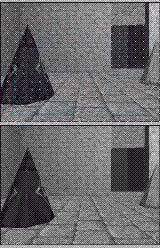
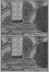
Below are two more examples of optical flow fields:
Note that almost all of the needles on the ground
are non-match cases. This is because the texture on the ground is too fine-grained
and gets lost in the gaussian filtering.
Back to top
Balance Strategy
The balance strategy is a control law that can be used
by mobile agents to avoid obstacles, to trail moving targets, or to escape
from approaching enemies [2]. In order to manage all
of these goals, the mobile agent should try to balance the amount of image
intensity change on the left and right sides of the center of its field
of view. In order to do this, the agent can determine the direction and
the magnitude of its rotation by looking at the difference of the sum of
the magnitudes of the left and right side optical flow vectors.
If the agent wants to avoid obstacles, then it should
turn away from the side that shows more motion, since this indicates a
possible approach to a stationary obstacle. An example of this case is
shown in the figure below:
 |
In this case, the sum of the magnitudes of
the flow vectors on the left side is greater than the right side sum. Therefore
the agent should turn right to avoid the obstacle. |
Similarly, if the agent wants to trail a target, it
should turn to the same side that shows more motion. In this way, it keeps
the target in focus.
A simple modification makes use of this strategy
in escaping from enemies. The agent simply moves backward, while keeping
the enemy in focus as in trailing a target.
Back to top
Time To Contact Estimation
The estimation of the remaining time to contact with
a surface is another useful tool for autonomous navigation, which can be
computed using optical flow fields [2]. When the agent
moves at a constant speed, the TTC can be estimated by the ratio of the
distance of a point in the image plane from the focus of expansion to the
rate of change in this distance (divergence from the focus of expansion)
[1][6].This
gives us the number of remaining frames before a contact to that point
takes place. The incorporation of the agent speed and the frame rate converts
this estimate from the dimensionless remaining number of frames to the
remaining seconds.
 |
This is a snapshot of our program in action
computing time to contact estimations. The image sequence used is prerecorded
by our robot while it was approaching a wall covered with newspapers with
a speed of 8 cm/sec (The newspapers provide a texture that is more adequate
for patch matching than the white, textureless wall). There are 76 frames
in this sequence.
In order to reduce the effect of input noise, or
the errors that may occur due to the integer nature of the needle lengths,
our program averages over a large number of estimates to determine the
overall single result. |
 |
This graph shows each of the time to contact estimations
made by the above run of our program for all of the successive frame pairs
in the input stream. |
Back to top
Our Test Domains
We test our programs both in simulated environments,
and in real environments by using a physical robot:
 |
We use Crystal Space, a free 3-D engine as
the basis for our simulated environments. It is developed in C++. For more
information about Crystal Space, click on the logo, or follow the link
below:
Crystal Space |
 |
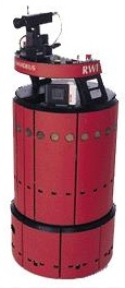
Our robot, Erik, is an indoor robot (RWI
- B21r) equipped with a digital 1/2" CCD color camera with digital signal
processing capabilities. You can learn more about Erik by clicking on his
images or by clicking the following link:
Erik (RWI - B21r) |
 |
 |
For more information about our camera, click on the image or
follow the link below:
TMC - 7DSP |
Back to top
Current Test Results
The following videos show the current performance of
our algorithms in both simulated and real environments:
 |
Erik is finding its way between chairs
in our laboratory using the balance strategy for obstacle avoidance. |
 |
Erik is running down the corridor, again
using the balance strategy. Note that this video is produced with a frame
rate of 3 frames per second, therefore please adjust your mpeg player program
accordingly to see the real motion. |
 |
Virtual Erik is wandering in a simulated environment
created by Crystal Space engine. |
 |
Another simulated environment. Virtual Erik is passing through a door,
and following a corridor. |
Back to top
References
[1] Ted A. Camus, ``Real-Time Optical Flow'', Ph.D. Thesis,
May 1995.
[2] Andrew P. Duchon, William H. Warren, and Leslie
Pack Kaelbling, ``Ecological Robotics'', Adaptive Behavior, Volume 6, Number
3/4, 1998.
[3] Marr, D., and Hildreth, E.C., ``Theory of Edge
Detection'', RoyalP(B-207), 1980, pp. 187-217.
[4] Nishihara, H. K., ``Practical Real-Time Imaging
Stereo Matcher'', OptEng(23), No. 5, September/October 1984, pp. 536-545.
[5] Nishihara, H. K., ``Real-Time Implementation
of a Sign-Correlation Algorithm for Image-Matching'', Technical report,
Teleos Research, February 1990.
[6] N. Ancona and T. Poggio, ``Optical Flow from
1D Correlation: Application to a Simple Time-to-Crash Detector'', In: Proceedings
of the Fourth International Conference on Computer Vision, Berling, Germany,
May 1993.
Back to top
Selim Temizer
Massachusetts Institute of Technology
Department of Electrical Engineering and Computer Science
The Artificial Intelligence Laboratory
Learning and Intelligent Systems (LIS) Group