VGG Convolutional Neural Networks Practical

This is an Oxford Visual Geometry Group computer vision practical, authored by Andrea Vedaldi and Andrew Zisserman, and modified for a BCS Computational Topics Tutorial by Phillip Isola. (An unmodified version of the tutorial is here.)

Convolutional neural networks are an important class of learnable representations applicable, among others, to numerous computer vision problems. Deep CNNs, in particular, are composed of several layers of processing, each involving linear as well as non-linear operators, that are learned jointly, in an end-to-end manner, to solve a particular tasks. These methods are now the dominant approach for feature extraction from audiovisual and textual data.

This practical explores the basics of learning (deep) CNNs. The first part introduces typical CNN building blocks, such as ReLU units and linear filters, with a particular emphasis on understanding back-propagation. The second part looks at learning two basic CNNs. The first one is a simple non-linear filter capturing particular image structures, while the second one is a network that recognises typewritten characters (using a variety of different fonts). These examples illustrate the use of stochastic gradient descent with momentum, the definition of an objective function, the construction of mini-batches of data, and data jittering. The last part shows how powerful CNN models can be downloaded off-the-shelf and used directly in applications, bypassing the expensive training process.

$$\newcommand{\bx}{\mathbf{x}} \newcommand{\by}{\mathbf{y}} \newcommand{\bz}{\mathbf{z}} \newcommand{\bw}{\mathbf{w}} \newcommand{\cP}{\mathcal{P}} \newcommand{\cN}{\mathcal{N}} \newcommand{\vc}{\operatorname{vec}}$$

Getting started

Download the code and data here.

Open and edit the script exercise1.m in the MATLAB editor. The script contains commented code and a description for all steps of this exercise, for Part I of this document. You can cut and paste this code into the MATLAB window to run it, and will need to modify it as you go through the session. Other files exercise2.m, exercise3.m, and exercise4.m are given for Part II, III, and IV.

Each part contains several Questions (that require pen and paper) and Tasks (that require experimentation or coding) to be answered/completed before proceeding further in the practical.

Sections that can safely be skipped are marked as "optional". These sections have bluish gray text and a gray background.

Part 1: CNN building blocks

Part 1.1: convolution

A feed-forward neural network can be thought of as the composition of number of functions
$$f(\bx) = f_L(\dots f_2(f_1(\bx;\bw_1);\bw_2)\dots),\bw_{L}).$$
Each function $f_l$ takes as input a datum $\bx_l$ and a parameter vector $\bw_l$ and produces as output a datum $\bx_{l+1}$. While the type and sequence of functions is usually handcrafted, the parameters $\bw=(\bw_1,\dots,\bw_L)$ are learned from data in order to solve a target problem, for example classifying images or sounds.

In a convolutional neural network data and functions have additional structure. The data $\bx_1,\dots,\bx_n$ are images, sounds, or more in general maps from a lattice1 to one or more real numbers. In particular, since the rest of the practical will focus on computer vision applications, data will be 2D arrays of pixels. Formally, each $\bx_i$ will be a $M \times N \times K$ real array of $M \times N$ pixels and $K$ channels per pixel. Hence the first two dimensions of the array span space, while the last one spans channels. Note that only the input $\bx=\bx_1$ of the network is an actual image, while the remaining data are intermediate feature maps.

The second property of a CNN is that the functions $f_l$ have a convolutional structure. This means that $f_l$ applies to the input map $\bx_l$ an operator that is local and translation invariant. Examples of convolutional operators are applying a bank of linear filters to $\bx_l$.

In this part we will familiarise ourselves with a number of such convolutional and non-linear operators. The first one is the regular linear convolution by a filter bank. We will start by focusing our attention on a single function relation as follows:
$$f: \mathbb{R}^{M\times N\times K} \rightarrow \mathbb{R}^{M' \times N' \times K'}, \qquad \bx \mapsto \by.$$
Open the example1.m file, select the following part of the code, and execute it in MATLAB (right button > Evaluate selection or Shift+F7).

% Read an example image
x = imread('peppers.png') ;

% Convert to single format
x = im2single(x) ;

% Visualize the input x
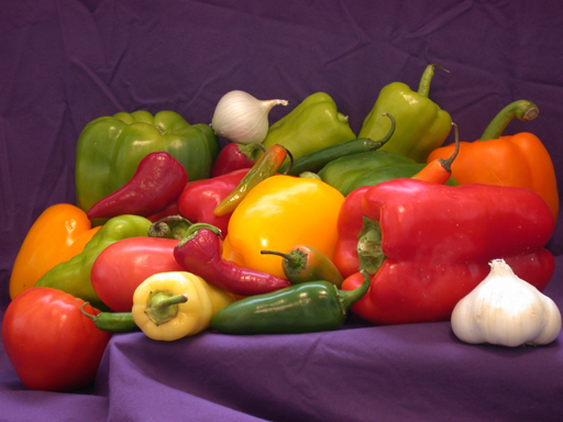
figure(1) ; clf ; imagesc(x) 

This should display an image of bell peppers in Figure 1:

Use MATLAB size command to obtain the size of the array x. Note that the array x is converted to single precision format. This is because the underlying MatConvNet assumes that data is in single precision.

Question. The third dimension of x is 3. Why?

Now we will create a bank 10 of $5 \times 5 \times 3$ filters.

% Create a bank of linear filters
w = randn(5,5,3,10,'single') ;

The filters are in single precision as well. Note that w has four dimensions, packing 10 filters. Note also that each filter is not flat, but rather a volume with three layers. The next step is applying the filter to the image. This uses the vl_nnconv function from MatConvNet:

% Apply the convolution operator
y = vl_nnconv(x, w, []) ;

Remark: You might have noticed that the third argument to the vl_nnconv function is the empty matrix []. It can be otherwise used to pass a vector of bias terms to add to the output of each filter.

The variable y contains the output of the convolution. Note that the filters are three-dimensional, in the sense that it operates on a map $\bx$ with $K$ channels. Furthermore, there are $K'$ such filters, generating a $K'$ dimensional map $\by$ as follows
$$y_{i'j'k'} = \sum_{ijk} w_{ijk} x_{i+i',j+j',k,k'}$$

Questions: Study carefully this expression and answer the following:

• Given that the input map $\bx$ has $M \times N \times K$ dimensions and that each of the $K'$ filters has dimension $M_f \times N_f \times K$, what is the dimension of $\by$?
• Note that $x$ is indexed by $i+i'$ and $j+j'$, but that there is no plus sign between $k$ and $k'$. Why?

Task: check that the size of the variable y matches your calculations.

We can now visualise the output y of the convolution. In order to do this, use the vl_imarraysc function to display an image for each feature channel in y:

% Visualize the output y
figure(2) ; clf ; vl_imarraysc(y) ; colormap gray ;

Question: Study the feature channels obtained. Most will likely contain a strong response in correspondences of edges in the input image x. Recall that w was obtained by drawing random numbers from a Gaussian distribution. Can you explain this phenomenon?

So far filters preserve the resolution of the input feature map. However, it is often useful to downsample the output. This can be obtained by using the stride option in vl_nnconv:

% Try again, downsampling the output
y_ds = vl_nnconv(x, w, [], 'stride', 16) ;
figure(3) ; clf ; vl_imarraysc(y_ds) ; colormap gray ;

As you should have noticed in a question above, applying a filter to an image or feature map interacts with the boundaries, making the output map smaller by an amount proportional to the size of the filters. If this is undesirable, then the input array can be padded with zeros by using the pad option:

% Try padding
y_pad = vl_nnconv(x, w, [], 'pad', 4) ;
figure(4) ; clf ; vl_imarraysc(y_pad) ; colormap gray ;

Task: Convince yourself that the previous code’s output has different boundaries compared to the code that does not use padding. Can you explain the result?

In order to consolidate what has been learned so far, we will now design a filter by hand:

w = [0  1 0 ;
     1 -4 1 ;
     0  1 0 ] ;
w = single(repmat(w, [1, 1, 3])) ;
y_lap = vl_nnconv(x, w, []) ;

figure(5) ; clf ; colormap gray ;
subplot(1,2,1) ; 
imagesc(y_lap) ; title('filter output') ;
subplot(1,2,2) ;
imagesc(-abs(y_lap)) ; title('- abs(filter output)') ;

Questions:

• What filter have we implemented?
• How are the RGB colour channels processed by this filter?
• What image structure are detected?

Part 1.2: non-linear gating

As we stated in the introduction, CNNs are obtained by composing several different functions. In addition to the linear filters shown in the previous part, there are several non-linear operators as well.

Question: Some of the functions in a CNN must be non-linear. Why?

The simplest non-linearity is obtained by following a linear filter by a non-linear gating function, applied identically to each component (i.e. point-wise) of a feature map. The simplest such function is the Rectified Linear Unit (ReLU)
$$y_{ijk} = \max\{0, x_{ijk}\}.$$
This function is implemented by vl_relu; let’s try this out:

w = single(repmat([1 0 -1], [1, 1, 3])) ;
w = cat(4, w, -w) ;
y = vl_nnconv(x, w, []) ;
z = vl_nnrelu(y) ;

figure(6) ; clf ; colormap gray ;
subplot(1,2,1) ; vl_imarraysc(y) ;
subplot(1,2,2) ; vl_imarraysc(z) ;

Tasks:

• Run the code above and understand what the filter $\bw$ is doing.
• Explain the final result $\bz$.

Part 1.3: pooling

There are several other important operators in a CNN. One of them is pooling. A pooling operator operates on individual feature channels, coalescing nearby feature values into one by the application of a suitable operator. Common choices include max-pooling (using the max operator) or sum-pooling (using summation). For example, max-pooling is defined as:
$$y_{ijk} = \max \{ y_{i'j'k} : i \leq i' < i+p, j \leq j' < j + p \}$$
Max pooling is implemented by the vl_nnpool function. Try this now:

y = vl_nnpool(x, 15) ;
figure(6) ; clf ; imagesc(y) ;

Question: look at the resulting image. Can you interpret the result?

The function vl_nnpool supports subsampling and padding just like vl_nnconv. However, for max-pooling feature maps are padded with the value $-\infty$ instead of 0. Why?

rho = 5 ;
kappa = 0 ;
alpha = 1 ;
beta = 0.5 ;
y_nrm = vl_nnnormalize(x, [rho kappa alpha beta]) ;
figure(6) ; clf ; imagesc(y_nrm) ;

Part 2: back-propagation and derivatives

The parameters of a CNN $\bw=(\bw_1,\dots\bw_L)$ should be learned in such a manner that the overall CNN function $\bz = f(\bx;\bw)$ achieves a desired goal. In some cases, the goal is to model the distribution of the data, which leads to a generative objective. Here, however, we will use $f$ as a regressor and obtain it by minimising a discriminative objective. In simple terms, we are given:

• examples of the desired input-output relations $(\bx_1,\bz_1), \dots, (\bx_n,\bz_n)$ where $\bx_i$ are input data and $\bz_i$ corresponding output values;
• and a loss $\ell(\bz,\hat\bz)$ that expresses the penalty for predicting $\hat\bz$ instead of $\bz$.

We use those to write the empirical loss of the CNN $f$ by averaging over the examples:
$$L(\bw) = \frac{1}{n} \sum_{i=1}^n \ell(\bz_i, f(\bx_i;\bw))$$
Note that the composition of the function $f$ with the loss $\ell$ can be though of as a CNN with one more layer (called a loss layer). Hence, with a slight abuse of notation, in the rest of this part we incorporate the loss in the function $f$ (which therefore is a map $\mathcal{X}\rightarrow\mathbb{R}$) and do not talk about it explicitly anymore.

The simplest algorithm to minimise $L$, and in fact one that is used in practice, is gradient descent. The idea is simple: compute the gradient of the objective $L$ at a current solution $\bw^t$ and then update the latter along the direction of fastest descent of $L$:
$$\bw^{t+1} = \bw^{t} - \eta_t \frac{\partial f}{\partial \bw}(\bw^t)$$
where $\eta_t \in \mathbb{R}_+$ is the learning rate.

Since $f$ is a composition of many functions (the layers in the network), its derivative can be calculated via the chain rule. Back-propagation is an algorithm that efficiently implements this calculation. More details are given in Section 2.1 below, but please see the notes here for simpler, more intuitive explanation.

Part 2.1: using back-propagation in practice

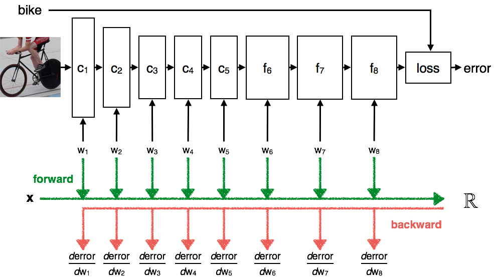
A key feature of MatConvNet and similar neural network packages is the ability to support gradient descent via back-propagation. In order to do so, lets focus on a single computational block $f$, followed by a function $g$, which represents all subsequent layers of the network:
$$\bx \longrightarrow \underset{\displaystyle\underset{\displaystyle\bw}{\uparrow}}{\boxed{f}} \longrightarrow \by \longrightarrow \boxed{g} \longrightarrow z$$
where $z$ is assumed to be a scalar. The way back-propagation works is you iteratively propagate "errors" backwards through the network. At each iteration of the algorithm, you have already computed the derivative for the tail of the network, $g$. This derivative is $\partial z / \partial \by$. Then to propagate the derivative back just one more layer you just multiple by the derivatives of this one additional layer, as specified by the chain rule.

Then each computation block (for example vl_nnconv or vl_nnpool) computes $\partial z / \partial \bx$ and $\partial z / \partial \bw$ given as input $\bx$, $\bw$, and $\partial z / \partial \by$. Let’s put this into practice:

% Read an example image
x = im2single(imread('peppers.png')) ;

% Create a bank of linear filters and apply them to the image
w = randn(5,5,3,10,'single') ;
y = vl_nnconv(x, w, []) ;

% Create the derivative dz/dy
dzdy = randn(size(y), 'single') ;

% Back-propagation
[dzdx, dzdw] = vl_nnconv(x, w, [], dzdy) ;

Task: Run the code above and check the dimensions of dzdx and dzdy. Does this matches your expectations?

An advantage of this modular view is that new building blocks can be coded and added to the architecture in a simple manner. However, it is easy to make mistakes in the calculation of complex derivatives. Hence, it is a good idea to verify results numerically. Consider the following piece of code:

% Check the derivative numerically
ex = randn(size(x), 'single') ;
eta = 0.0001 ;
xp = x + eta * ex  ;
yp = vl_nnconv(xp, w, []) ;

dzdx_empirical = sum(dzdy(:) .* (yp(:) - y(:)) / eta) ;
dzdx_computed = sum(dzdx(:) .* ex(:)) ;

fprintf(...
  'der: empirical: %f, computed: %f, error: %.2f %%\n', ...
  dzdx_empirical, dzdx_computed, ...
  abs(1 - dzdx_empirical/dzdx_computed)*100) ;

Questions:

• What is the meaning of ex in the code above?
• What are the derivatives dzdx_empirical and dzdx_computed?

Tasks:

• Run the code and convince yourself that vl_nnconv derivatives is (probably) correct.
• Create a new version of this code to test the derivative calculation with respect to $\bw$.

We are now ready to build our first elementary CNN, composed of just two layers, and to compute its derivatives:

% Parameters of the CNN
w1 = randn(5,5,3,10,'single') ;
rho2 = 10 ;

% Run the CNN forward
x1 = im2single(imread('peppers.png')) ;
x2 = vl_nnconv(x1, w1, []) ;
x3 = vl_nnpool(x2, rho2) ;

% Create the derivative dz/dx3
dzdx3 = randn(size(x3), 'single') ;

% Run the CNN backward
dzdx2 = vl_nnpool(x2, rho2, dzdx3) ;
[dzdx1, dzdw1] = vl_nnconv(x1, w1, [], dzdx2) ;

Question: Note that the last derivative in the CNN is dzdx3. Here, for the sake of the example, this derivative is initialised randomly. In a practical application, what would this derivative represent?

We can now use the same technique as before to check that the derivative computed through back-propagation are correct.

% Check the derivative numerically
ew1 = randn(size(w1), 'single') ;
eta = 0.0001 ;
w1p = w1 + eta * ew1  ;

x1p = x1 ;
x2p = vl_nnconv(x1p, w1p, []) ;
x3p = vl_nnpool(x2p, rho2) ;

dzdw1_empirical = sum(dzdx3(:) .* (x3p(:) - x3(:)) / eta) ;
dzdw1_computed = sum(dzdw1(:) .* ew1(:)) ;

fprintf(...
  'der: empirical: %f, computed: %f, error: %.2f %%\n', ...
  dzdw1_empirical, dzdw1_computed, ...
  abs(1 - dzdw1_empirical/dzdw1_computed)*100) ;

Part 3: learning a tiny CNN

In this part we will learn a very simple CNN. The CNN is composed of exactly two layers: a convolutional layer and a max-pooling layer:
$$\bx_2 = W * \bx_1 + b, \qquad \bx_3 = \operatorname{maxpool}_\rho \bx_2.$$
$W$ contains a single $3\times 3$ square filter, so that $b$ is a scalar. and the input image $\bx=\bx_1$ has a single channel.

Task

• Open the file tinycnn.m and inspect the code. Convince yourself that the code computes the CNN just described.
• Look at the paddings used in the code. If the input image $\bx_1$ has dimensions $M\times N$, what is the dimension of the output feature map $\bx_3$?

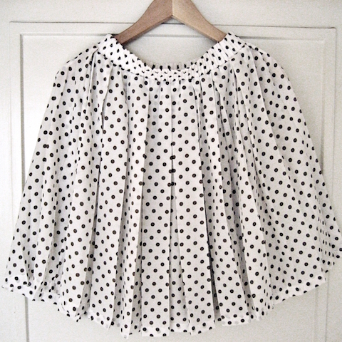
In the rest of the section we will learn the CNN parameters in order to extract blob-like structures from images, such as the ones in the following image:

Part 3.1: training data and labels

The first step is to load the image data/dots.jpg and to use the supplied extractBlackBlobs function to extract all the black dots in the image.

% Load an image
im = rgb2gray(im2single(imread('data/dots.jpg'))) ;

% Compute the location of black blobs in the image
[pos,neg] = extractBlackBlobs(im) ;

The arrays pos and neg contain now pixel labels and will be used as annotations for the supervised training of the CNN. These annotations can be visualised as follows:

figure(1) ; clf ; 
subplot(1,3,1) ; imagesc(im) ; axis equal ; title('image') ;
subplot(1,3,2) ; imagesc(pos) ; axis equal ; title('positive points (blob centres)') ;
subplot(1,3,3) ; imagesc(neg) ; axis equal ; title('negative points (not a blob)') ;
colormap gray ; 

Task: Inspect pos and neg and convince yourself that:

• pos contains a single true value in correspondence of each blob centre;
• neg contains a true value for each pixel sufficiently far away from a blob.

Are there pixels for which both pos and neg evaluate to false?

Part 3.2: image preprocessing

Before we attempt to train the CNN, the image is pre-processed to remove its mean value. It is also smoothed by applying a Gaussian kernel of standard deviation 3 pixels:

% Pre-smooth the image
im = vl_imsmooth(im,3) ;

% Subtract median value
im = im - median(im(:)) ;

We will come back to this preprocessing steps later.

Part 3.3: learning with gradient descent

We will now setup a learning problem to learn $W$ and $b$ to detect black blobs in images. Recall that the CNN computes for each image pixel $(u,v)$ a score $f(\bx;\bw,b)_{(u,v)}$. We would like this score to be:

• at least as large as 1 for any pixel that is marked as a blob centre (pos or $(u,v)\in\cP$) and
• at most zero for any pixel that is marked as being far away from a blob (neg or $(u,v)\in\cN$).

We do so by defining and then optimising the following objective function:
$$E(\bw,b) = \frac{\lambda}{2}\|\bw\|^2 + \frac{1}{|\cP|}\sum_{(u,v) \in \cP} \max\{0, 1 - f(\bx;\bw,b)_{(u,v)}\} + \frac{1}{|\cN|}\sum_{(u,v) \in \cN} \max\{0, f(\bx;\bw,b)_{(u,v)}\}.$$

Questions:

• What can you say about the score of each pixel if $\lambda=0$ and $E(\bw,b) =0$?
• Note that the objective enforces a margin between the scores of the positive and negative pixels. How much is this margin?

We can now train the CNN by minimising the objective function with respect to $\bw$ and $b$. We do so by using an algorithm called gradient descent with momentum. Given the current solution $(\bw_t,b_t)$ and update it , this is updated to $(\bw_{t+1},b_t)$ by following the direction of fastest descent as given by the negative gradient $-\nabla E(\bw_t,b_t)$ of the objective. However, gradient updates are smoothed by considering a momentum term $(\bar\bw_{t}, \bar\mu_t)$, yielding the update equations
$$\bar\bw_{t+1} \leftarrow \mu \bar\bw_t + \eta \frac{\partial E}{\partial \bw_t}, \qquad \bw_{t+1} \leftarrow \bw_{t} - \bar\bw_t.$$
and similarly for the bias term. Here $\mu$ is the momentum rate and $\eta$ the learning rate.

Questions:

• Explain why the momentum rate must be smaller than 1. What is the effect of having a momentum rate close to 1?
• The learning rate establishes how fast the algorithm will try to minimise the objective function. Can you see any problem with a large learning rate?

The parameters of the algorithm are set as follows:

numIterations = 500 ;
rate = 5 ;
momentum = 0.9 ;
shrinkRate = 0.0001 ;
plotPeriod = 10 ;

Tasks:

• Inspect the code in the file exercise3.m. Convince yourself that the code is implementing the algorithm described above. Pay particular attention at the forward and backward passes as well as at how the objective function and its derivatives are computed.
• Run the algorithm and observe the results. Then answer the following questions:
  
  • The learned filter should resemble the discretisation of a well-known differential operator. Which one?
  • What is the average of the filter values compared to the average of the absolute values?
• Run the algorithm again and observe the evolution of the histograms of the score of the positive and negative pixels in relation to the values 0 and 1. Answer the following:
  
  • Is the objective function minimised monotonically?
  • As the histograms evolve, can you identify at least two “phases” in the optimisation?
  • Once converged, do the score distribute in the manner that you would expect?

Hint: the plotPeriod option can be changed to plot the diagnostic figure with a higher or lower frequency; this can significantly affect the speed of the algorithm.

Part 4: learning a character CNN

In this part we will learn a CNN to recognise images of characters.

Part 4.1: prepare the data

Open up exercise4.m and execute Part 4.1. The code loads a structure imdb containing images of the characters a, b, …, z rendered using approximately 931 fonts downloaded from the Google Fonts Project. Look at the imdb.images substructure:

>> imdb.images
ans = 
       id: [1x24206 double]
     data: [32x32x24206 single]
    label: [1x24206 double]
      set: [1x24206 double]

These are stored as the array imdb.images.id is a 24,206-dimensional vector of numeric IDs for each of the 24,206 character images in the dataset. imdb.images.data contains a $32 \times 32$ image for each character, stored as a slide of a $32\times 32\times 24,\!206$-dimensional array. imdb.images.label is a vector of image labels, denoting which one of the 26 possible characters it is. imdb.images.set is equal to 1 for each image that should be used to train the CNN and to 2 for each image that should be used for validation.

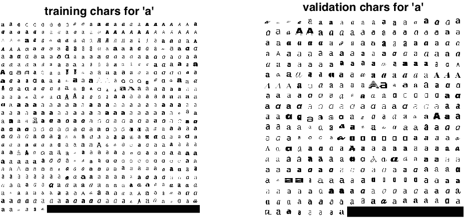
Task: look at the Figure 1 generated by the code and at the code itself and make sure that you understand what you are looking at.

Part 4.2: intialize a CNN architecture

The function initializeCharacterCNN.m creates a CNN initialised with random weights that will be trained to recognise character images.

Tasks:

1. By inspecting initializeCharacterCNN.m get a sense of the architecture that will be trained. How many layers are there? How big are the filters?
2. Use the function vl_simplenn_display to produce a table summarising the architecture.

Note that the penultimate layer has 26 output dimensions, one for each character. Character recognition looks at the maximal output to identify which character is processed by the network.

However, the last network layer is vl_nnsoftmaxloss, which in turn is a combination of the vl_nnsoftmax function and of the classification log-loss vl_nnloss. The softmax operator is given by
$$y_{ijk'} = \frac{e^{x_{ijk'}}}{\sum_{k} e^{x_{ijk}}}$$
whereas the log-loss is given by
$$y_{ij} = - \log x_{ij c_{ij}}$$
where $c_{ij}$ is the index of the ground-truth class at spatial location $(i,j)$.

Remark: While in MatConvNet all operators are convolutional, in this case the network is configured such that the output of the classification layer is a $1 \times 1 \times 26$-dimensional feature map, i.e. there remains only one spatial location.

Tasks:

1. Understand what the softmax operator does. Hint: to use the log-loss the data must be in the (0, 1] interval.
2. Understand what is the effect of minimising the log-loss. Which neural response should become larger?
3. Why do you think MatConvNet provides a third function vl_nnsoftmaxloss combining both functions into a single layer?

Part 4.3: train and evaluate the CNN

We are now ready to train the CNN. To this end we use the example SGD implementation in MatConvNet (examples/cnn_train.m). This function requires some options:

trainOpts.batchSize = 100 ;
trainOpts.numEpochs = 100 ;
trainOpts.continue = true ;
trainOpts.useGpu = false ;
trainOpts.learningRate = 0.001 ;
trainOpts.numEpochs = 15 ;
trainOpts.expDir = 'data/chars-experiment' ;

This says that the function will operate on SGD mini-batches of 100 elements, it will run for 15 epochs (passes through the data), it will continue from the last epoch if interrupted, if will not use the GPU, it will use a learning rate of 0.001, and it will save any file in the data/chars-experiment subdirectory.

Before the training starts, the average image value is subtracted:

% Take the average image out
imageMean = mean(imdb.images.data(:)) ;
imdb.images.data = imdb.images.data - imageMean ;

This is similar to what we have done in Part 3.

The training code is called as follows:

% Call training function in MatConvNet
[net,info] = cnn_train(net, imdb, @getBatch, trainOpts) ;

Here the key, in addition to the trainOpts structure, is the @getBatch function handle. This is how cnn_train obtains a copy of the data to operate on. Examine this function (see the bottom of the exercise4.m file):

function [im, labels] = getBatch(imdb, batch)
im = imdb.images.data(:,:,batch) ;
im = 256 * reshape(im, 32, 32, 1, []) ;
labels = imdb.images.label(1,batch) ;

The function extracts the $m$ images corresponding to the vector of indexes batch. It also reshape them as a $32\times 32\times 1\times m$ array (as this is the format expected by the MatConvNet functions) and multiplies the values by 256 (the resulting values match the network initialisation and learning parameters). Finally, it also returns a vector of labels, one for each image in the batch.

Task: Run the learning code and examine the plots that are produced. As training completes answer the following questions:

1. How many images per second can you process? (Look at the output in the MATLAB screen)
2. There are two sets of curves: energy and prediction error. What do you think is the difference? What is the “energy”?
3. Some curves are labelled “train” and some other “val”. Should they be equal? Which one should be lower than the other?
4. Both the top-1 and top-5 prediction errors are plotted. What do they mean? What is the difference?

Once training is finished, the model is saved back:

% Save the result for later use
net.layers(end) = [] ;
net.imageMean = imageMean ;
save('data/chars-experiment/charscnn.mat', '-struct', 'net') ;

Note that we remember the imageMean for later use. Note also that the softmaxloss layer is removed from the network before saving.

Part 4.4: visualise the learned filters

The next step is to glance at the filters that have been learned:

figure(2) ; clf ; colormap gray ;
vl_imarraysc(squeeze(net.layers{1}.filters),'spacing',2)
axis equal ;
title('filters in the first layer') ;

Task: what can you say about the filters?

Part 4.5: apply the model

We now apply the model to a whole sequence of characters. This is the image data/sentence-lato.png:

% Load the CNN learned before
net = load('data/chars-experiment/charscnn.mat') ;

% Load the sentence
im = im2single(imread('data/sentence-lato.png')) ;
im = 256 * (im - net.imageMean) ;

% Apply the CNN to the larger image
res = vl_simplenn(net, im) ;

Question: The image is much wider than 32 pixels. Why can you apply to it the CNN learned before for $32\times 32$ patches?

Task: examine the size of the CNN output using size(res(end).x). Does this match your expectation?

Now use the decodeCharacters() function to visualise the results:

% Visualize the results
figure(3) ; clf ;
decodeCharacters(net, imdb, im, res) ;

Tasks: inspect the output of the decodeCharacters() function and answer the following:

1. Is the quality of the recognition any good?
2. Does this match your expectation given the recognition rate in your validation set (as reported by cnn_train during training)?

Part 5: using pretrained models

A characteristic of deep learning is that it constructs representations of the data. These representations tend to have a universal value, or at least to be applicable to an array of problems that transcends the particular task a model was trained for. This is fortunate as training complex models requires weeks of works on one or more GPUs or hundreds of CPUs; these models can then be frozen and reused for a number of additional applications, with no or minimal additional work.

In this part we will see how MatConvNet can be used to download and run high-performance CNN models for image classification. These models are trained from 1.2M images in the ImageNet datasets to discriminate 1,000 different object categories.

Several pertained models can be downloaded from the MatConvNet website, including several trained using other CNN implementations such as Caffe. One such models is included in the practical data/imagenet-vgg-verydeep-16.mat file. This is one of the best models from the ImageNet ILSVCR Challenge 2014.

Part 5.1: load a pre-trained model

The first step is to load the model itself. This is in the format of the vl_simplenn CNN wrapper, and ships as a MATLAB .mat file:

net = load('data/imagenet-vgg-verydeep-16.mat') ;
vl_simplenn_display(net) ;

Tasks:

1. Look at the output of vl_simplenn_display and understand the structure of the model. Can you understand why it is called “very deep”?
2. Look at the size of the file data/imagenet-vgg-verydeep-16.mat on disk. This is just the model.

Part 5.2: use the model to classify an image

We can now use the model to classify an image. We start from peppers.png, a MATLAB stock image:

% obtain and preprocess an image
im = imread('peppers.png') ;
im_ = single(im) ; % note: 255 range
im_ = imresize(im_, net.normalization.imageSize(1:2)) ;
im_ = im_ - net.normalization.averageImage ;

The code normalises the image in a format compatible with the model net. This amounts to: converting the image to single format (but with range 0,…,255 rather than [0, 1] as typical in MATLAB), resizing the image to a fixed size, and then subtracting an average image.

It is now possible to call the CNN:

% run the CNN
res = vl_simplenn(net, im_) ;

As usual, res contains the results of the computation, including all intermediate layers. The last one can be used to perform the classification:

% show the classification result
scores = squeeze(gather(res(end).x)) ;
[bestScore, best] = max(scores) ;

figure(1) ; clf ; imagesc(im) ;
title(sprintf('%s (%d), score %.3f',...
  net.classes.description{best}, best, bestScore)) ;

That completes this practical.

Links and further work

• The code for this practical is written using the software package MatConvNet. This is a software library written in MATLAB, C++, and CUDA and is freely available as source code and binary.
• The ImageNet model is the VGG very deep 16 of Karen Simonyan and Andrew Zisserman.

Acknowledgements

• Beta testing by Karel Lenc and Carlos Arteta.

History

• Used in the Oxford AIMS CDT, 2014-15.