Planning Algorithms for Bicycles
As you may have already surmised from checking out parts of my website, I really like bicycles! So, for my final project in 6.832 (Underactuated Robotics, taught by Prof. Russ Tedrake), I decided to apply some of the techniques we’ve been learning about to different simplified planar models of bicycle dynamics. Specifically, I used the following randomized sampling motion-planning algorithms: (RRT, RG-RRT, and LQR-RRT*. RRT and RRT* have been used successfully for a variety of motion planning tasks, and tend to work great for holonomic systems. However, for systems with more complicated dynamics or systems with differential constraints, RRT tends to expand its tree inefficiently due to inaccurate distance and extension metrics. The performance of RRT* is also very sensitive to these metrics. LQR-RRT* attempts to ameliorate these difficulties by linearizing points in the RRT and constructing locally optimal LQR controllers to use for the distance and extension heuristics. As the tree gets bigger and more densely covers state space, these approximations become more and more accurate.
Bicycle Models
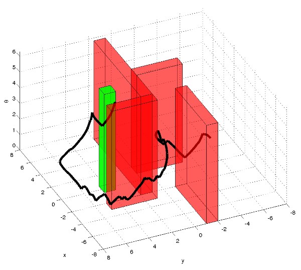
I looked primarily at three different bicycle models, increasing in complexity. The first is the Dubin’s vehicle, which has a three-dimensional state space. This vehicle is modeled as a point that moves with constant velocity and whose angle can be steered via a control input. Since the vehicle cannot instananeously move laterally, this is a simple model for a bicycle. Planning output from an RRT planning for this Dubin’s model is shown in the picture at right, where the axes represent x, y, and theta. The red blocks are obstacles that must be manuevered about, and the green box is the goal region.
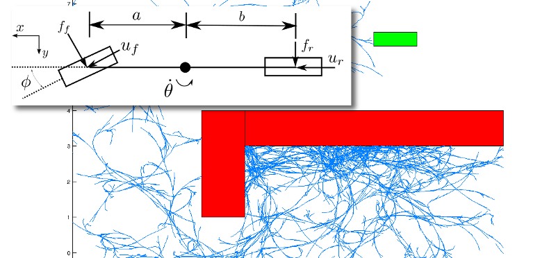
After the Dubin’s model, I looked at a slightly more complicated version with a four dimensional state space. This model allowed the bicycle to accelerate and decelerate (no more constant velocity requirements), as well as had a more realistic steering control. The wheels are modeled as having “directional friction” - infinite laterally parallel to the axis, and 0 going forward and backward. Put another way, there is a differential constraint that the bicycle wheels cannot slip laterally.
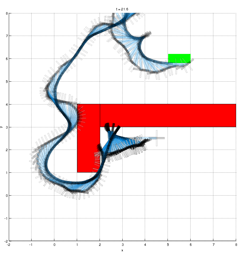
Finally, the most complicated planar model I examined was a slipping bicycle that had a seven-dimensional state space. Please see the details in my paper, but this bicycle modeled the planar physics accurately, and also allowed the wheels to skid. A good analogy for this is a bicycle riding on sand. The top image shows a solution for this bicycle, as does the video below.
Algorithms
I predominantly used RRT (Rapidly-exploring Random Tree), RG-RRT (reachability-guided RRT), and LQR-RRT* to plan for these bicycle models. RRT works well for many holonomic systems, but often has trouble for systems with dynamics. RG-RRT and LQR-RRT* attempt to solve this difficulty using two different approaches.
RG-RRT works by restricting the expansion of the tree into only yet-unexplored areas of state space. Any sample that is too close to the existing tree is rejected. In this way, the tree is kept small and is restricted to expand in new directions, even if there is not a very good distance or extension metric being used. RG-RRT implements this by augmenting a normal RRT with Reachable nodes, which represent the extrema of control inputs applied to the current states. By comparing the distances of randomly sampled notes to these Reachable nodes and to the normal nodes in the tree, it is possible to reject samples that don’t really do much new exploring.
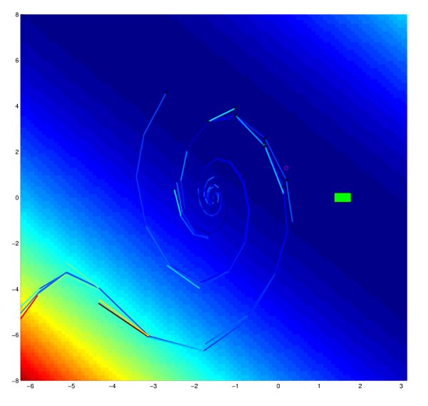
LQR-RRT* takes a completely different approach. Instead of forcefully rejecting samples, LQR-RRT* attempts to improve the distance and extension heuristics so that they work better for dynamical systems. Namely, these heuristics are approximated by locally optimal linearizations of the state space about nodes in the tree using an LQR controller. An intermediate screenshot of this is shown in the picture at right.
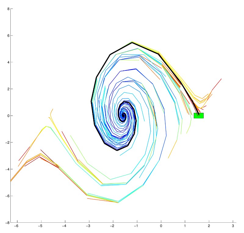
Interestingly, I found that LQR was not applicable to a number of my bicycle models. It turns out that my Dubin’s model had a linearization that was not controllable, and the seven-dimensional state space model for the slipping bicycle exhibited this same phenomena in certain conditions (namely, when there was no lateral force on the tires). Therefore, applying LQR-RRT* to these models was difficult. I was able to apply it to the inverted pendulum (which is, admittedly, not a bicycle!). The results for this are shown at right.
Paper
For more information, please see my final paper.
Video
Here’s a video of RG-RRT planning for the bicycle model, and the resulting solution:
