Supplement for "SimpleFlow: A Non-iterative, Sublinear Optical Flow Algorithm"
EUROGRAPHICS 2012
Michael Tao, Jiamin Bai, Pushmeet Kohli, Sylvain Paris
Architectural Considerations
How we compare with other algorithms
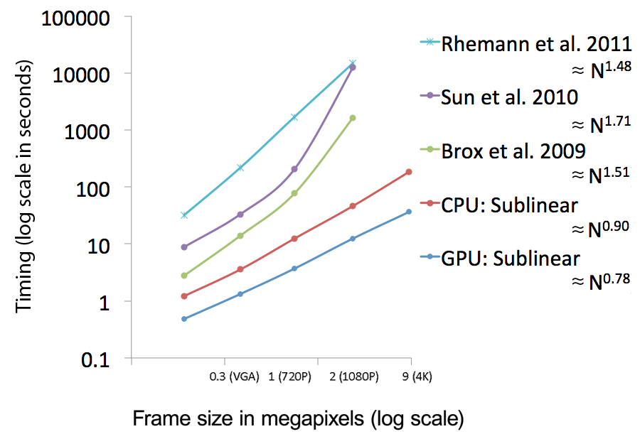 |
Log-log plot of the running times with respect to
the video size. Comparative to other algorithms, we perform
at a sublinear computational time relative to number pixels
while others compute at nonlinear rates. We stopped timings
for Rhemann et al. [2011], Sun et al. [2010], and Brox et al. [2009]
because they took too long to complete at 4K resolutions.
CPU implementation is computed on an Intel i7 920 2.66GHz, 4 cores, 8GB RAM. GPU implementation is computed on a NVIDIA GTX 285 1GB RAM. |
Our pipeline
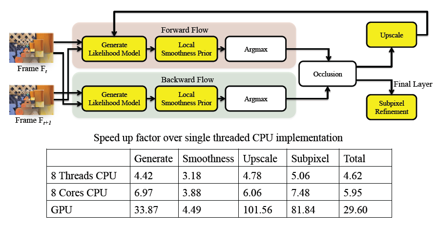 |
Illustrating different stages of our pipeline. Stages highlighted in yellow are parallelized. We tabulate the speed up factor of the 8 threads CPU implementation and the GPU implementation against the single thread CPU implementation for various stages as well as the whole pipeline. |
Break Down
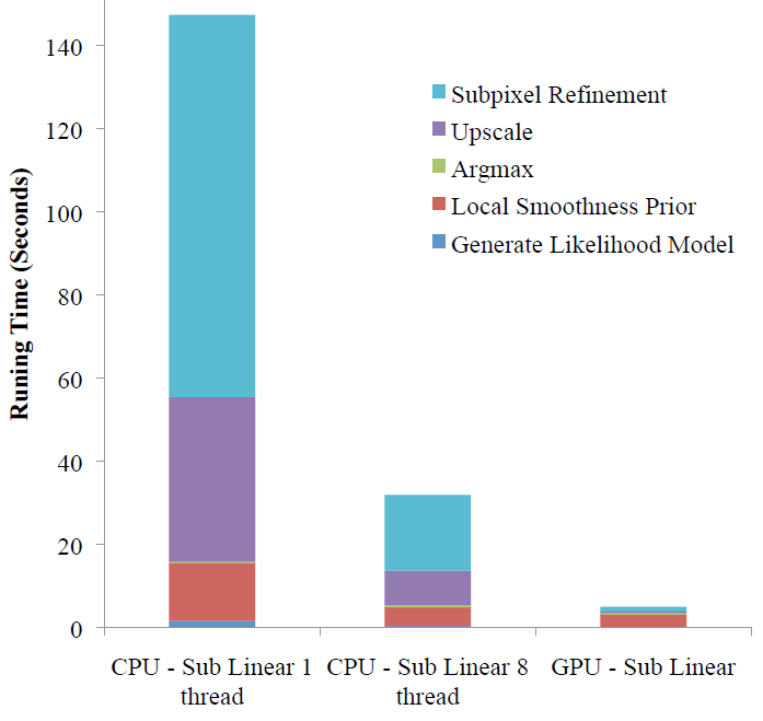 |
This shows the breakdown of timings for difference stages across 3 implementations. We can see that while most stages attain reasonable speed ups, Local Smoothing Model does not scale as well. |
GPU vs CPU
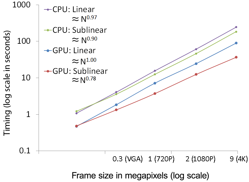 |
Log-log plot of the running times with respect to the video size. Here shows how our algorithm exploits parallelized architecture such as the GPU. Our sublinear method performs better on the GPU and most importantly yields a practical complexity on the order of ~N^78 (in blue). |
CPU Cores vs. Threads
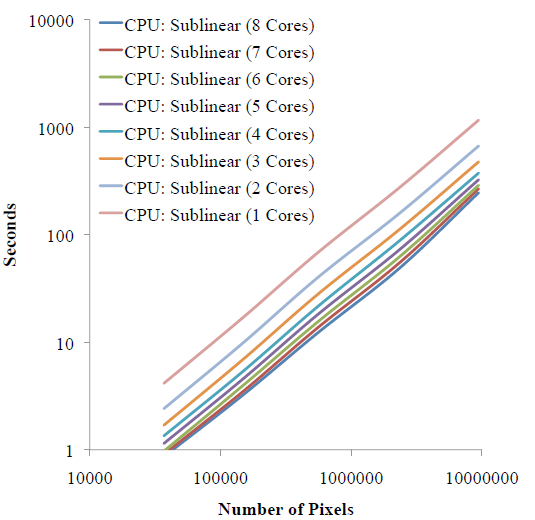 |
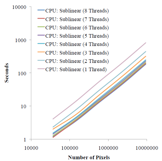 |
| Here we show log-log plots of timings as we scale the image size for varies number of threads on the Intel i7 machine. The timings scale monotonically with image size and the performance benefits for increasing threads decreases. This is because there are only 4 physical cores on the machine. |
Here we show log-log plots of timings as we scale the image size for varies number of threads on the Intel Xeon machine. The timings scale monotonically with image size and the performance benefits for increasing cores decreases. However, because we have 8 physical cores, the performance is better than 8 threads on the Intel i7 machine with simultaneous multithreading. |
Bilateral Likelihood Map Filtering
Input Images
Frame 1

|
Frame 2
 |
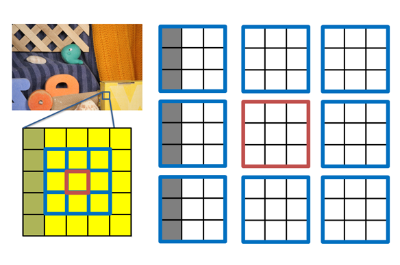
Likelihood Map
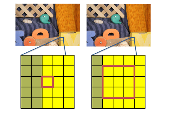
To obtain the likelihood map, for each pixel, we find the difference between the pixel at (x,y) from frame 1 with the neighborhood around pixel (x,y).

The likelihood map is shown on the right, where we can see the likelihood is all white because all its neighborhoods are also yellow. This brings us ambiguity where the pixel went from frame 1 to 2.
The Bilateral Likelihood Map Filtering
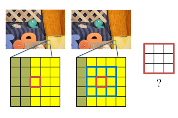
To correct the problem, we look at the likelihood map of its neighbors.
Here, we can use a simple averaging scheme which weights the filter by distance and color similarity.
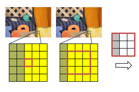
Now, we have an output likelihood map that tells us more information than before. Here, we can generally see pixels should move towards the right.
<< back to main menu (click here)