 |
Modeling the shape of the scene: a holistic representation of the spatial envelopeAude Oliva, Antonio TorralbaInternational Journal of Computer Vision, Vol. 42(3): 145-175, 2001. PDF |
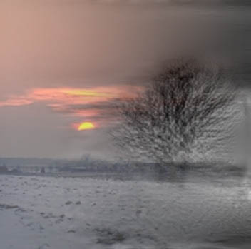
Abstract: In this paper, we propose a computational model of the recognition of real world scenes that bypasses the segmentation and the processing of individual objects or regions. The procedure is based on a very low dimensional representation of the scene, that we term the Spatial Envelope. We propose a set of perceptual dimensions (naturalness, openness, roughness, expansion, ruggedness) that represent the dominant spatial structure of a scene. Then, we show that these dimensions may be reliably estimated using spectral and coarsely localized information. The model generates a multidimensional space in which scenes sharing membership in semantic categories (e.g., streets, highways, coasts) are projected closed together. The performance of the spatial envelope model shows that specific information about object shape or identity is not a requirement for scene categorization and that modeling a holistic representation of the scene informs about its probable semantic category.
This material is based upon work supported by the National Science Foundation under CAREER Grant No. 0546262. Any opinions, findings, and conclusions or recommendations expressed in this material are those of the author(s) and do not necessarily reflect the views of the National Science Foundation.
GIST Descriptor (Matlab code)
Download:
Download all the matlab code and examples here: gistdescriptor.zipComputing the gist descriptor:
To compute the gist descriptor on an image use the function LMgist. The next example reads one image and computes the descriptor (the images demo1.jpg and demo2.jpg are available inside the gistdescriptor.zip file).
% Load image
img = imread('demo2.jpg');
% GIST Parameters:
clear param
param.orientationsPerScale = [8 8 8 8]; % number of orientations per scale (from HF to LF)
param.numberBlocks = 4;
param.fc_prefilt = 4;
% Computing gist:
[gist, param] = LMgist(img, '', param);
Visualization:
To visualize the gist descriptor use the function showGist.m. Here there is an example of how to use it:
% Visualization
figure
subplot(121)
imshow(img)
title('Input image')
subplot(122)
showGist(gist, param)
title('Descriptor')
Image similarities:
When computing image similarities, it might be important to normalize the image size before computing the GIST descriptor. This can be achieved by setting the image size inside the param struct (using the field param.imageSize). The LMgist function will resize and crop each image to match the specified size before computing the gist descriptor. The resizing operation will not affect the aspect ratio of the original image. The crop will be centered and the image will be resize so that the cropped region preserves as much as possible from the original input image. Here is an example:
% Load images
img1 = imread('demo1.jpg');
img2 = imread('demo2.jpg');
% GIST Parameters:
clear param
param.imageSize = [256 256]; % it works also with non-square images (use the most common aspect ratio in your set)
param.orientationsPerScale = [8 8 8 8]; % number of orientations per scale
param.numberBlocks = 4;
param.fc_prefilt = 4;
% Computing gist:
gist1 = LMgist(img1, '', param);
gist2 = LMgist(img2, '', param);
% Distance between the two images:
D = sum((gist1-gist2).^2)
Image collections:
The first call to LMgist will precompute the filters in the frequency domain and store them in param.G, subsequent calls will be faster.
% GIST Parameters:
clear param
param.imageSize = [256 256]; % set a normalized image size
param.orientationsPerScale = [8 8 8 8]; % number of orientations per scale (from HF to LF)
param.numberBlocks = 4;
param.fc_prefilt = 4;
% Pre-allocate gist:
Nfeatures = sum(param.orientationsPerScale)*param.numberBlocks^2;
gist = zeros([Nimages Nfeatures]);
% Load first image and compute gist:
img = imread(file{1});
[gist(1, :), param] = LMgist(img, '', param); % first call
% Loop:
for i = 2:Nimages
img = imread(file{i});
gist(i, :) = LMgist(img, '', param); % the next calls will be faster
end
The script demoGist.m shows a few more examples and also how it works with non-square images. The function LMgist can also work the LabelMe toolbox.
8 Scene Categories Dataset
|
Download: Images.zip, Annotations.zip and example.m This dataset contains 8 outdoor scene categories: coast, mountain, forest, open country, street, inside city, tall buildings and highways. There are 2600 color images, 256x256 pixels. All the objects and regions in this dataset have been fully labeled. There are more than 29.000 objects. The annotations are available in LabelMe format. For a newer and more challenging scene recognition benchmark, use the SUN database or the Places database. |
|||||||||||||||||||||||||||||||||||||||||||||||||||||||||||||||||||||||||||||||||
|
Scene recognition Results training with 100 samples per class using an SVM classifier with a gaussian kernel, test on the rest. Average on the diagonal is 83.7%
|

Related publications
Scene and place recognition
Context-based vision system for place and object recognition
A. Torralba, K. P. Murphy, W. T. Freeman and M. A. Rubin
IEEE Intl. Conference on Computer Vision (ICCV), Nice, France, October 2003.
Project
page
Contextual priming for object detection
A. Torralba
International Journal of Computer Vision, Vol. 53(2), 169-191, 2003.
Project
page
Depth estimation from image structure
A. Torralba, A. Oliva
IEEE Transactions on Pattern Analysis and Machine Intelligence, Vol. 24(9): 1226-1238. 2003.
Contextual Guidance of Attention in Natural scenes: The role of Global features on object search
A. Torralba, A. Oliva, M. Castelhano and J. M. Henderson
Psychological Review. Vol 113(4) 766-786, Oct, 2006.
Project page