A Simple Constant Acceleration Controller

The contents of this post came out of helping my little brother design a controller for use on his FIRST robotics team. It requires a little bit of simple calculus but should be accessible to all high school students that understand what a derivative and integral are.

Why Constant Acceleration Controller?

When driving a physical system to a particular setpoint (for example moving a robot arm to a particular angle, or moving a robot drivetrain 6 inches forward) we often want to limit the acceleration the system undergoes. Acceleration is often directly proportional to the tractive force, current required to drive the motor and/or forces experienced by the system. We often want to limit acceleration to prevent slippage, avoid popping a fuse, damaging electronics or damaging mechanical components of our system. Limiting acceleration directly, however, can reduce the performance of our system by never allowing to exceed the limit even briefly.

Designing a controller that targets a specific acceleration can help mitigate the issue. Controllers designed with acceleration in mind can also be very effective in systems with a lot of mechanical play and slop. If the direction of the acceleration doesn’t change the system usually behaves as if it has no slop. This can yield a very noticeable increase in performance in systems with large amounts of play.

Controller Designing

Outline

First we’re going to derive the motion profile (graph of position and speed vs time) that we want our system to follow. Then we’re going to decide how we want our controller to respond to deviations from this optimal motion profile. This will lead to some simple formulas that you can run on your very own robot.

Motion Profile

Lets say that we want to accelerate at acceleration \(a_0\) from a starting velocity of \(-v_0\). Assume for now that we turn the robot off when the velocity hits zero.

Integration gives us that the velocity is \(v(t) = -v_0 + a_0 t\), and the below plot of velocity versus time.

Integrating again gives us position versus time \(x(t) = -v_0 t + \frac{a_0}{2} t^2\).

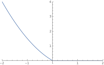
Note that the position versus time is parabolic. The robot will be move slow close to the goal and fast far away. This is usually how we want our robot to behave—we really only need precision at the very end of our motions.

Controller Design

While the simplest motor controllers usually only allow you to a duty cycle, my little brother’s team had already developed a velocity controller for their system. Back when I was on the team we ran a filtered, feed-forward, PI loop on top of some code that remapped outputs as to linearize the response of the motors. However, a tuned PID loop on velocity is a good start.

We’re going to take advantage of the fact that the velocity controller has already been tuned and tested in order to reduce the number of tuning parameters we have across our system. Our controller’s job will to compute the target velocity as a function of our position.

$v(t) = a_0 t$ $x(t) = \frac{a_0}{2} t^2$

We can compute \(v(x)\), the function that computes the target velocity as a function of position by solving for \(x\) and substituting.

$t = \sqrt{\frac{2}{a_0} x}$ $v(x) = a_0 \sqrt{\frac{2}{a_0} x} = \sqrt{2 a_0 x}$

And voila! Using the formula for \(v(x)\) we can easily compute the desired target velocity and get a controller that targets a constant acceleration.

Further Notes

It’s pretty important that you have a well-tuned velocity control loop for this controller to work. Also since the robot takes some time to react, this controller can cause the velocity to be a bit higher than desired. This issue can be resolved by either simply turning down the desired acceleration or adding an integral compensator.

This controller can be quite aggressive near the target position, which can cause issues if your system is close to oscillating.