
 The percentage of BCM vehicles in the mixed traffic
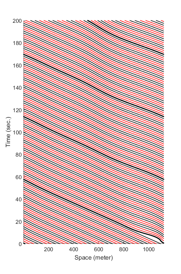
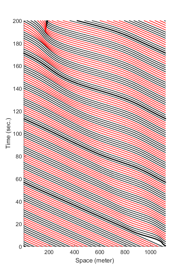
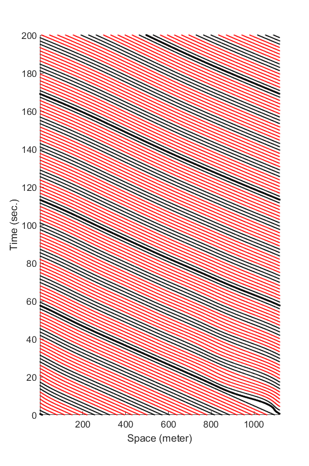
Fig.4: The mixed traffic when \(K = 5\) and \(L = 3\), where \(K\) denotes the number of cars in each CFM chain and \(L\) denotes the number of cars in each BCM chain.

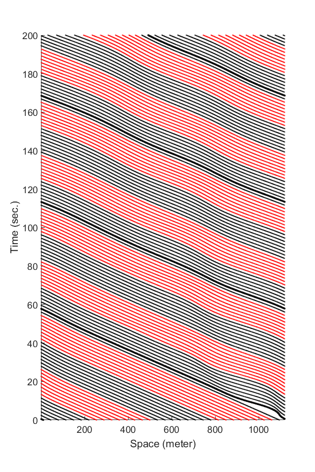
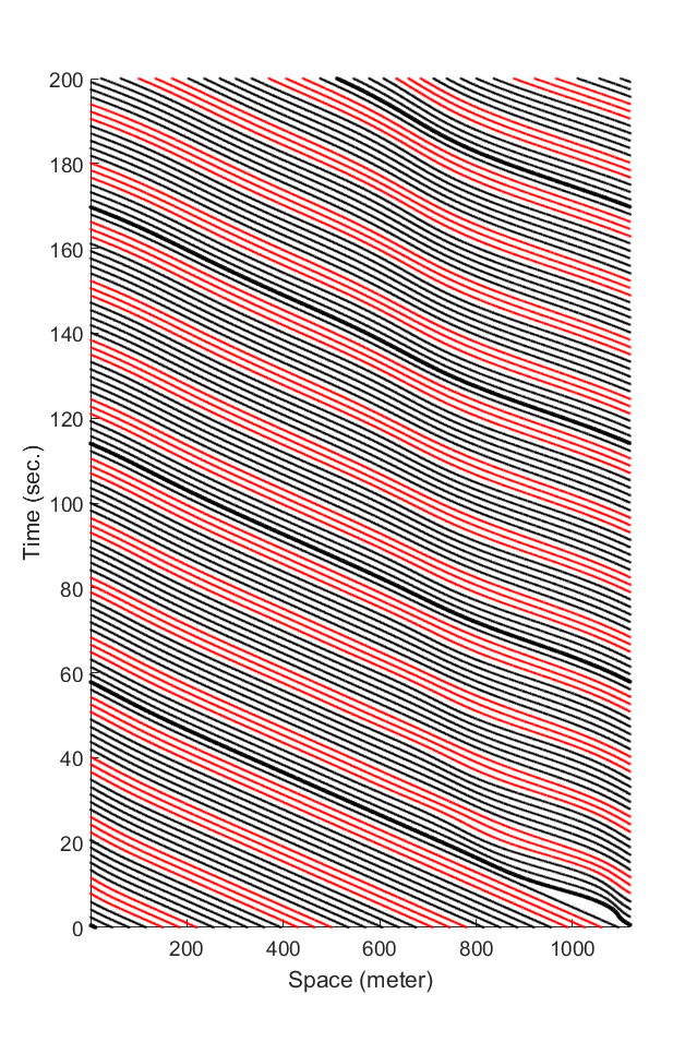
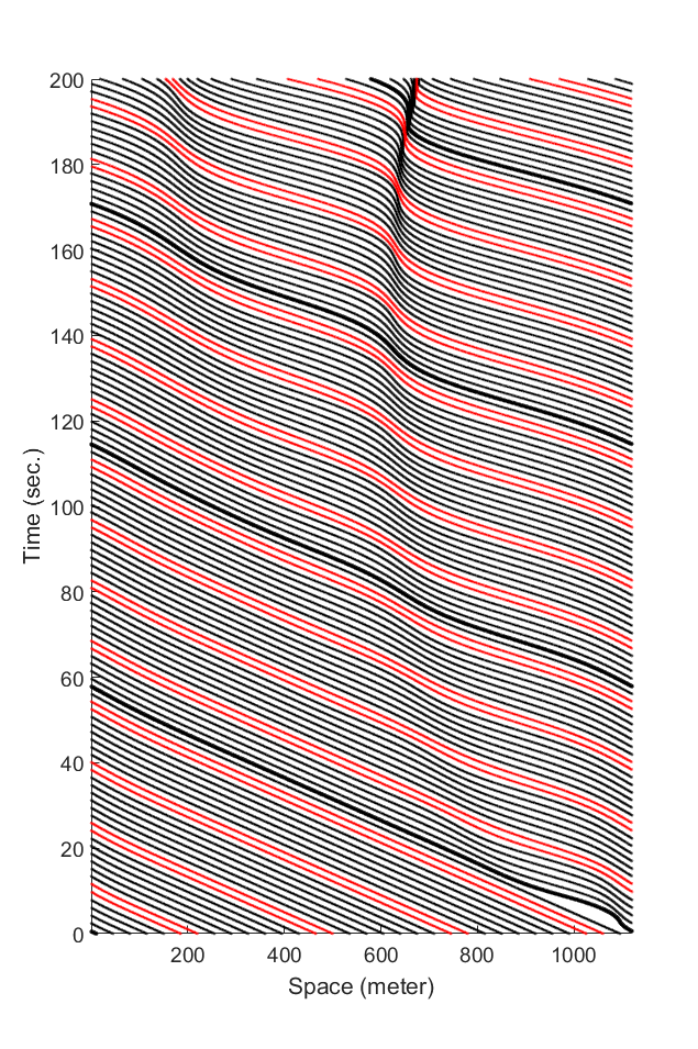
Fig.5: The mixed traffic when \(K = 3\) and \(L = 5\), where \(K\) denotes the number of cars in each CFM chain and \(L\) denotes the number of cars in each BCM chain.

 The distribution of BCM cars (i.e., concentrated or dispersed).