6.869 problem set one

max van kleek

6.869 problem set one

february 24, 2005

download all solution code here:
http://people.csail.mit.edu/~emax/6.869/ps1/max-ps1.code.zip

problem one

part a)

function [alpha, beta, theta, u0, v0, R, t] = calibrate(f2D,f3D)
%% 
%% computes the intrinsic (camera) and extrinsic (world) parameters
%% given real-world coordinates in homogenous coords (f3D) of some
%% item in space, and corresponding pixel locations in f2d
%%

M = projM(f2D,f3D) % first estimate the projection matrix

% M = (A b)
A = M(:,[1:3]);
b = M(:,4);
% then recover the parameters
a1 = A(1,:)'; a2 = A(2,:)'; a3 = A(3,:)';

% eqtns 3.11 in forsythe + ponce
rho = 1/sqrt(sum(a3.^2))
r3 = rho * a3
u0 = rho.^2 * (a1' * a3)
v0 = rho.^2 * (a2' * a3);

% equations 3.13 in forsythe + ponce
theta = acos( -(cross(a1, a3)'*cross(a2,a3)) / ( sqrt(sum(cross(a1,a3).^2)) * sqrt(sum(cross(a2,a3).^2)) ) );
alpha = rho.^2 * sqrt(sum(cross(a1,a3).^2))*sin(theta);
beta = rho.^2 *  sqrt(sum(cross(a2,a3).^2))*sin(theta);

% eqtns 3.14 in forsythe + ponce
r1 = rho ^2 * sin(theta) / beta * cross(a2,a3);
r2 = cross(r3,r1);

R = [r1'; r2'; r3']
K = [alpha -alpha*cot(theta) u0; 0 beta/sin(theta) v0; 0 0 1]; %rho * A * inv(R);
t = rho * inv(K)*b;

results:

  [alpha beta theta u0 v0 R t] = calibrate(f2D,f3D);

alpha =
   1.1177e+03
beta =
   1.1177e+03
theta =
    1.5708
u0 =
   300.5000
v0 =
  300.4991
R =
    0.7071    0.0000   -0.7071
   -0.4150    0.8097   -0.4150
    0.5725    0.5869    0.5725
t =
   -0.0000
    0.0810
   -6.9277

part b)

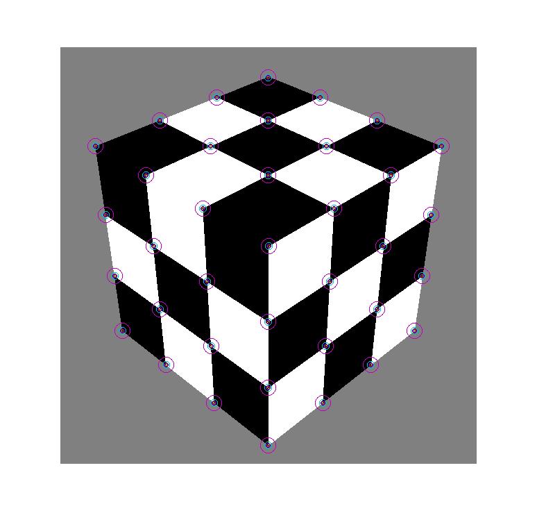
function f2D = pcamview(f3D, alpha, beta, theta, u0, v0, R, t) 
% projects f3D onto a plane according to the given extrinsic
% and intrinsic parameters

f2D = [];
for p = f3D,
   
   %% from 2.17 in forsythe and ponce
   
   M(1,[1:3]) = alpha*R(1,:) - alpha * cot(theta) * R(2,:) + u0 * R(3,:);
   M(2,[1:3]) = beta/sin(theta)*R(2,:) + v0*R(3,:);
   M(3,[1:3]) = R(3,:);
   
   M(1,4) = alpha*t(1) - alpha*cot(theta)*t(2) + u0*t(3);
   M(2,4) = beta/sin(theta)*t(2) + v0*t(3);
   M(3,4) = t(3);
   
   %% from 2.16 in forsythe and ponce
   
   z = M(3,:)*p
   u = (M(1,:)*p)/(z)
   v = (M(2,:)*p)/(z)
   
   f2D = [f2D [u v]'];
end

result:

  >> pcamview(f3D,alpha,beta,theta,u0,v0,R,t)

ans =

  300.5000  574.0207
  300.5000  490.9958
  300.5000  396.3433
  300.5000  287.4363
  222.4527  512.7543
  217.6516  430.9434
  212.2211  338.4075
  206.0288  232.8895
  152.7584  458.0450
  144.1846  377.6910
  134.5544  287.4362
  123.6596  185.3304
   90.1441  408.8933
   78.5908  330.1454
   65.6946  242.2448
   51.2069  143.4970
  549.7931  143.4970
  477.3404  185.3304
  394.9712  232.8895
  457.2591  106.4140
  383.5976  143.4970
  300.5000  185.3304
  374.6685   73.3157
  300.5000  106.4140
  217.4024  143.4970
  300.5000   43.5927
  226.3315   73.3157
  143.7409  106.4140
  535.3054  242.2448
  466.4456  287.4362
  388.7789  338.4075
  522.4092  330.1454
  456.8154  377.6910
  383.3484  430.9434
  510.8559  408.8933
  448.2416  458.0450
  378.5473  512.7543

problem two

part a)

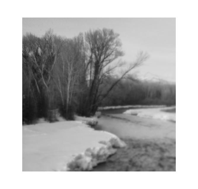
The maximum acuity according to the acutiy limit equation (a=0.23e+0.7) would be when the eccentricity, e=0. At this point, we get an acuity of 0.7. Half of the acuity here would correspond to twice this value, or 1.4. Using simple trigonometry, we have an image with X pixels per side, adding up to a length D, and stand from a distance 2D. The angle that the image makes with our eye occurs at half the acuity limit, 1.4 minutes, or 1.4*1/60 degrees. Therefore we have the relation

  tan (1.4*1/60) = d/x * 1/(2d)

the d's cancel, leaving us:

  x = 1/(2*tan (1.4*1/60))
  x = 2455/2 = 1228 pixels per side

part b

Here we want a function, d_spacing(i,j), that will give us the pixel spacing corresponding to half the maximum acuity for any coordinate expressed in the units given in this problem. The assumption still holds that we are standing 2 units away from the image, and the image is 1 unit by 1 unit. In order to do this, we first need to compute the eccentricity at (i,j). Using simple trignonometry,

e(i,j) = atan(sqrt( ((i/X).^2 +(j/X)^2))/2 )

where X represents the number of pixels per side. Now, we need to compute d_view, which is the distance to the point at which we are looking

d_view = sqrt(4 + (i/X)^2 + (j/X).^2 )

Now, d_spacing is simply the arc inscribed by the angle corresponding to the limit of half the maximum visual acuity, given at a distance of d_view.

d_spacing = d_view * tan((0.23*(e(i/j)*180/PI)+0.7) * 1/60 * pi/180))

The scale factors (1/60*pi/180) above need to exist in order to convert the "minutes" values back to radians.

part c)

In order to determine what level of a gaussian pyramid to use, we equate the d_spacing expression above to 2^n/X, since 2^n/X represents the width of each pixel in a gaussian pyramid of n levels, for an image with X pixels and unit (1x1) size. Then, we solve for n:

2^n/X = d_view * tan((0.23*(e(i/j)*180/PI)+0.7) * 1/60 * pi/180))

yields:

n = log2(X * d_view * tan((0.23*(e(i/j)*180/PI)+0.7) * 1/60 * pi/180))

I implemented this as a function in matlab as follows:

function n = nlevels(x, y, WIDTH)
% computes number of gaussian pyramid levels we need for problem 2 d

sx = x/WIDTH; sy = y/WIDTH;

e = atan(0.5*sqrt(sx^2+sy^2));
a = 0.23 * e*(180/pi) + 1.4;
dview = sqrt(sx^2 + sy^2 + 4);
n = log2(WIDTH * dview * tan (a/60 * pi/180));

part d)

function pi = pyramidit(img) img = img([1:1228],[1:1228]); % first generate the pyramids maxlvl = ceil(nlevels(size(img,1),size(img,2),size(img, 1)) + 1); [pyramids pyrsizes] = buildGpyr(img, maxlvl); % debugging size(pyramids) pyrsizes % % then upblur each one bpyr(:,:,1) = pyrBand(pyramids,pyrsizes,1); for py=2:maxlvl, % pull out the appropriate band pimg = pyrBand(pyramids,pyrsizes,py); % upsample blur = upBlur(pimg,py-1); % stash bpyr(:,:,py) = blur([1:1228],[1:1228]); end % now, reconstruct ourselves a new image pi = []; for i=1:size(img,1), for j = 1:size(img,2), lvl = nlevels(i,j,size(img,1)); mixing = (lvl - floor(lvl)); pyr1ij = (1-mixing)*bpyr(i,j,floor(lvl + 1)); pyr2ij = (mixing )* bpyr(i,j,ceil(lvl + 1)); pi(i,j) = pyr1ij + pyr2ij; end end imshow(pi);

result:

problem three

function synthIM = SynthTexture(sample, w, s)
% original texture sample

% initialize to a negative number so it's easy to distinguish between
% filled and unfilled
synthIM = -1*ones(s);
synthSize = s;

%% ====================== utility funcitons ========================
function b = isfilled(ijs)
    idxs = sub2ind(synthSize,ijs(:,1),ijs(:,2));
    b = ~(synthIM(idxs)==-1);
end

%% == findEmpty ==
function plist = findEmpty(synthIM, w) 
% finds boundary entries that need to be filled
% 

    % try converting to binary first then xor the difference
    
    simsize = size(synthIM);
    
    dilate = imdilate(synthIM,ones(3));
    dilthresh = threshzero(dilate);
    synthresh = threshzero(synthIM);
    edges = xor ( dilthresh, synthresh );
    
    ptlst = find(edges == 1.0); 
    [is js] = ind2sub(simsize,ptlst);
    is = is - floor(w/2);  js = js - floor(w/2);
    plist = [is'; js'];
    
    %% delete out of bounds points
    %% plist(:,min(plist,[],1)<=0)=[];
end
== end of findEmpty ==

== ValidMatrix.m ==
function validMatrix = makeValidMatrix(Sample,i,j,width)
%%  
%%  Constructs a ValidMatrix for a sample with upper-left
%%  corner (i,j) and width width

validMatrix = ones(width);
sample = getSample(Sample,i,j,width);

for ii=i:i+width-1,
  for jj=j:j+width-1,
    vi = ii-i+1;
    vj = jj-j+1;    

    %% boundary conditions
    if ( ii < 1 | jj < 1 | ii > size(Sample,1) | jj > size(Sample,2) )
      validMatrix(vi,vj)=0;
    end
    if(sample(vi,vj)<0)
      validMatrix(vi,vj)=0;
    end
  end
end

%% == end of makeValidMatrix ==

%% == SynthTexture main == 

%% pick a random wxw sample from sample and plop it in the middle
seedw = 3;

si = s(1)/2; sj = s(2)/2;
rsrci = 32 - floor(seedw/2); %-floor(w/2);  % floor(rand(1)*(size(sample,1)-seedw))+1;
rsrcj = 4 - floor(seedw/2);  %-floor(w/2); % floor(rand(1)*(size(sample,2)-seedw))+1;
synthIM(si:si+seedw-1,sj:sj+seedw-1) = ...
    sample(rsrci:rsrci+seedw-1,rsrcj:rsrcj+seedw-1);

figure(4);
testshow(synthIM);
figure(1);

%% =================================================================
% precompute a gaussian mask
sigma = w/6.4;
gmask = gauss2d(w,sigma);

% find things to fill
tofill = findEmpty(synthIM,w)

counter = 0; 
%% debugging 
disposed = 0;
%% end debugging
wmiddle = floor(w/2);

while ( length(find(synthIM<0)) > 0) % while we have unfilled pixels
  
  lengthtofill = length(tofill)
  for pt = tofill,
    %% what to do %% 
    pt_i = pt(1);  pt_j = pt(2);
    
    template = getSample(synthIM,pt_i,pt_j,w);
    validmask = makeValidMatrix(synthIM,pt_i,pt_j,w);
    G = validmask .* gmask;

    [bestmatches err] = findMatches(template,sample,G);
    
    % select one
    if (length(bestmatches) > 0)
      pick = floor(size(bestmatches,3)*rand(1))+1; %% pick one at random!
      bestmatch = bestmatches(:,:,pick);
      synthIM(pt_i + wmiddle, pt_j+wmiddle) = bestmatch(wmiddle+1,wmiddle+1);
      counter = counter+1;
    end
				 
  end
  tofill = findEmpty(synthIM,w);
 end
end

findMatches:

function [bestmatches, errors] = findMatches(template,sample,G)
% searches sample for template and returns the 

epsilon = 0.1;

sizeG = size(G);
sizetemplate = size(template);

w = size(template,1);
v = size(template,2);
%sigma = w/6.4;
%gmask = gauss2d(w,sigma);

total = sum(sum(G)); % find maximum by summing over the mask

SSD = [];
for i=1:(size(sample,1) - w),
    for j=1:(size(sample,2) - v),
        SSD(i,j) = sum(sum( ...
	    ((template-sample([i:i+w-1],[j:j+v-1])).^2 ) .* G));
    end
    SSD(i,j) = SSD(i,j)/total;
end

idxs = [];

while (length(idxs) == 0) 
  % minSSD cutoff -- 
  minSSD = min(SSD(:));
  idxs = find(SSD < min( DELTA, minSSD*(1+EPSILON)));
  EPSILON = EPSILON*1.1;
  DELTA=DELTA*1.1;
end

bestmatches = [];
errors = [];

if (length(idxs) > 0) 
    [i j] = ind2sub(size(SSD),idxs);
    for match=1:length(i)
      i_match = i(match);  j_match = j(match);
      bestmatches(:,:,match) = ...
	  sample([i_match:i_match+w-1],[j_match:j_match+v-1]);
      errors(match) = SSD(i_match,j_match);
    end 
   % bestmatches = sample([i:i+w-1],[j:j+v-1]);
end

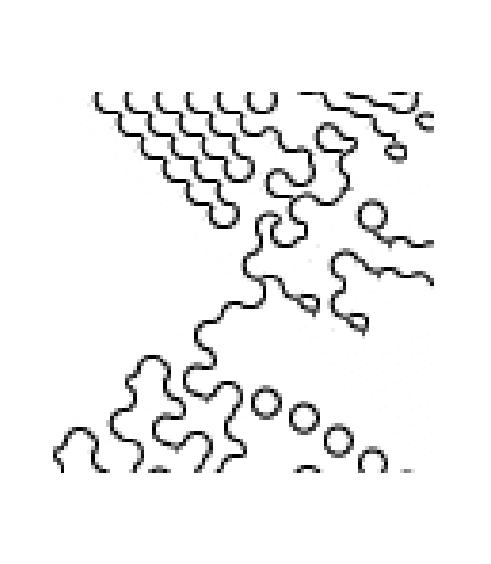
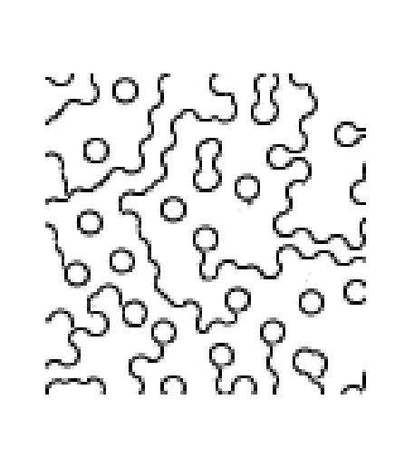
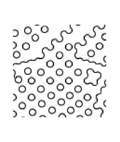
results: Each time we run the algorithm, even with the same window size, we will get different patterns due ot the random process we are employing to pick the best texture. Here are the set of pictures generated with EPSILON=0.001, which enforces most strict (optimal) choosing. starting with seed at (4,32), generating [100 100]:

window size = 5,
window size = 7

window size = 11

problem four

part a)

>> XYZ = [cx'; cy'; cz']*sA

ans =

    9.8584  
   11.6454
   11.7413

X -> 9.85
Y -> 11.64
Z -> 11.74

normalized coefficients X = x / (x + y + z) 
	Xnorm =   XYZ(1)/sum(XYZ) = 0.2965
	Ynorm =   XYZ(2)/sum(XYZ) = 0.3503
	Znorm =   XYZ(3)/sum(XYZ) = 0.3532

part b)

  
Given a signal represented with primaries P(450), P(550), P(650)
represent them in P(460) P(510) P(590)


  C = [cx'; cy'; cz'];
  
  % establish the primaries 
  
  P = zeros(length(cx),3);
  P((450-400)/5,1)=1;
  P((550-400)/5,2)=1;
  P((650-400)/5,3)=1;

  e = C*P'*[a b c]';

  % now, to find what combination we need in our new basis, compute C*Pnew
  % where Pnew is our new basis

  Pnew = zeros(length(cx),3);
  Pnew((460-400)/5,1)=1;
  Pnew((510-400)/5,2)=1;
  Pnew((590-400)/5,3)=1;
  
  C*Pnew*enew = C*P*e';
  enew = inv(C*Pnew)*C*P*[a b c]';

this matrix, inv(C*Pnew)*C*P has value:

>> inv(C*Pnew)*C*P

    1.0327   -0.1849    0.0456
   -0.0878    1.5790   -0.3771
    0.0196    0.4239    0.3548

part c)

So what we are trying to accomplish is to express each of the X, Y, Z
primaries as linear combinations of our own Primaries, P(460), P(510), and
P(640).

Therefore, what we'd like to do is this:

   eX = w1*eP1 + w2*eP2 + w3*eP3
   eY = w4*eP1 + w5*eP2 + w6*eP3
   eZ = w7*eP1 * w8*eP2 + w9*eP3

   or, more compactly

   [eX eY eZ]' = W * [eP1 eP2 eP3]'

   We want to find W.  Switching things around, we can write:

   [eP1 eP2 eP3]' = inv(W) * [eX eY eZ]';

   Fortunately, we already know inv(W), since this is the problem
   of representing an arbitary color (in this case our primaries)
   as combinations of X, Y, and Z.

   inv(W) = [cx'; cy'; cz']*[P1 P2 P3];

   where P1 = [ 0 0 ... 1 .. 0 ]'; corresponding to wavelength 450

   where P2 = [ 0 0 ... 0 .. 1 .. 0 ]'; corresponding to wavelength 510

   where P3 = [ 0 0 ... 0 .. 0 .. 1 .. 0 ]'; corresponding to wavelength 640


   thus, 

   inv(W) = [Cx(460) Cy(460) Cz(460); Cx(510) Cy(510) Cz(510); Cx(640) Cy(640) Cz(640)]; 

   inverting this back, we get inv(inv(W)) = W

   therefore, we have the relation

   [eX eY eZ]' = inv([cx';cy';cz']*[P1 P2 P3]) * [eP1 eP2 eP3]';

   the value inv([cx';cy';cz']*[P1 P2 P3]) for CIE XYZ and primaries 450, 510, and 640 are:


>> P1 = zeros(length(cx),1);
>> P2 = zeros(length(cx),1);
>> P3 = zeros(length(cx),1);
>> P1((450-400)/5,1) = 1;
>> P2((510-400)/5,1) = 1;    
>> P3((640-400)/5,1) = 1;
>> inv([cx'; cy'; cz']*[P1 P2 P3]) 

ans =

    0.1137   -0.2840    0.5435
   -0.9548    2.3844    0.1466
    1.7765    0.1719   -0.3498