Form a 3 dimensional cube of random pmf values between 0 and 1 for each triplet of states, normalized to integrate to one over a whole cube of data.
Make a random inital guess for your joint probabilities, P(a,b,c) and iterative modify it using IPF ofr 5 to 10 iterations.
Plot the fit of the observed marginals for several iterations of IPF. Also plot the KL distance between the original and estimated joint probailities as a function of IPF iteration.
function pmf = makeRandPmf()
  %% computes a random pmf for our cube, normalizing
  %% so that it integrates to 1
  pmf = rand([5 5 5]);
  pmf = pmf / sum(sum(sum(pmf)));
end;

function marg = marginalX(jointpmf)
  %% returns the marginal probability density of the PDF
  %% as a function of X (i.e., marginalizes over Y and Z)
   marg = sum(sum(jointpmf, 2),3);
end

function marg = marginalY(jointpmf)
  %% returns the marginal probability density of the PDF
  %% as a function of Y (i.e., marginalizes over X and Z)
   marg = shiftdim(sum(sum(jointpmf,1),3));
end

function marg = marginalZ(jointpmf)
  %% returns the marginal probability density of the PDF
  %% as a function of Z (i.e., marginalizes over X and Y)
   marg = shiftdim(sum(sum(jointpmf,1),2),2);
end;

function nextapprox = ipfIter(truemargX, truemargY, truemargZ, approxpmf, iteration),
   %% given our true observed marginals (truemargX, truemargY,
   %% truemargZ) and our current approximation for the pmf,
   %% computes the next approximation.  iteration is our iteration index

   nextapprox = [];
   amX = marginalX(approxpmf);
   amY = marginalY(approxpmf);
   amZ = marginalZ(approxpmf);
   for i=1:size(approxpmf,1),
     for j=1:size(approxpmf,2),
       for k=1:size(approxpmf,3),

           if mod(iteration,3) == 0,
               nextapprox(i,j,k) = approxpmf(i,j,k)*(truemargX(i)/amX(i));
           elseif mod(iteration,3) == 1,
               nextapprox(i,j,k) = approxpmf(i,j,k)*(truemargY(j)/amY(j));
           elseif mod(iteration,3) == 2,
               nextapprox(i,j,k) = approxpmf(i,j,k)*(truemargZ(k)/amZ(k));
           end;

       end;
     end;
   end;
end
results:
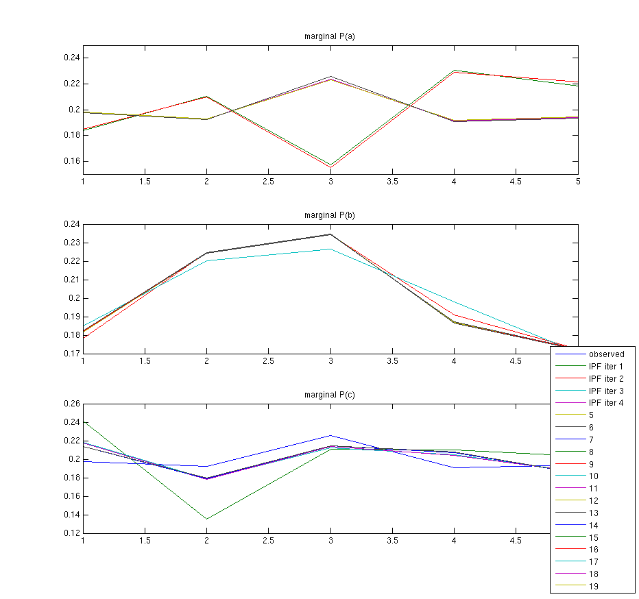
Plot of the marginals for each iteration of IPF until i=20
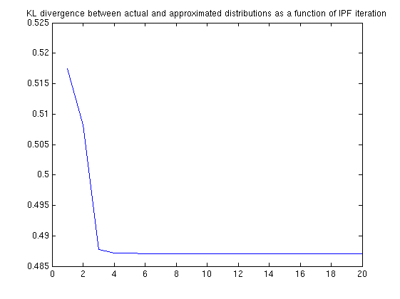
Plot of the KL difference between the final pdf and the original:
Slice plot of the actual PDFs:
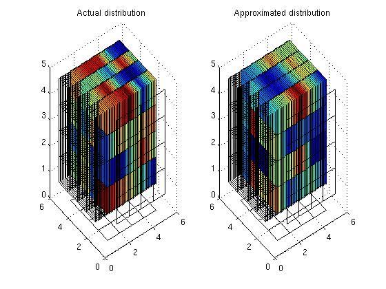
As can be seen in the pdf plots, the actual PDFs look quite different, even though their marginals converge within 4 iterations. It seems that this is our IPF algorithm getting stuck in a local optimum; our KL distance further supports this hypothesis (by not converging to 0). I am not sure how to "shake it loose".