max van kleek
6.869 advances in computer vision: learning and interfaces
problem set two
march 10, 2005
problem one
part one a)
the difference-of-gaussian is a function DoG(x, y, sigma, k) where:
- x,y - x,y-coord of point to be evaluated
- sigma - base standard deviation of the gaussian
- k - multiplicative factor for sigma to get the sigma for the next-level gaussian
or, equivalently could be defined as DoG(x, y, sigma1, sigma2):
- x,y - x,y-coord of point to be evaluated
- sigma1 - base standard deviation of the first gaussian
- sigma2 - base standard deviation of the second gaussian
part one b)
to speed up scale selection, the paper does two things:
- iterative blurring of layers
- Instead of blurring each layer with the appropriate (k^n)*sigma,
which would require a large gaussian (blur) kernel and thus would
be computationally expensive, we perform an iterative blurring,
taking the image at a particular blur and convolving it with sigma_delta
(defined next) to yield the next level. Sigma_delta is effectively much
smaller than (k^n)*sigma, therefore the convolution is efficient.
- downsampling every octave
- Instead of generating the image layers used to make DoG layers at all scales,
the paper only generates image layers corresponding to the levels between a
given sigma to twice that sigma. Then, to generate the next (and successive)
octaves, the existing image layer generated for the current octave corresponding
to 2*sigma is downsampled to half its original resolution - a very fast operation,
and the process repeated.
part one c)
Using the gaussian semi-group property we want to find an expression for g(sigma_delta):
- g(sigma_delta^2) * (g(sigma_cur^2) * I) = g((k*sigma_cur)^2) * I
- setup: We want to find a sigma_delta which we can convolve with
an image blurred with a gaussian of variance (sigma_cur^2) to
get an image blurred at k^2 * sigma_cur^2.
- g(sigma_delta^2) * (g(sigma_cur^2) * I) = g((k*sigma_cur)^2) * I
- convolution is associative!
- g(sigma_delta^2 + sigma_cur^2) * I = g((k*sigma_cur)^2) * I
- use semi-group property
- sigma_delta^2 + sigma_cur^2 = (k*sigma_cur)^2
- now we can concentrate on the inside
- sigma_delta = sqrt((k*sigma_cur)^2 - sigma_cur^2)
- isolating terms..
- sigma_delta = sigma_cur*sqrt(k^2 - 1)
keypoint detector code:
compute_dog_points
function Points = compute_dog_points(Image)
%% computes difference-of-gaussian keypoints on Image

   function sd = sigmadelta(k,sigma_cur)
   %% returns the sigma_delta (what we need to convolve with to
   %% achieve an blur of k more than sigma_cur
      sd = sigma_cur*sqrt(k.^2-1);
   end;

%% retrieves parameters from get_dog_params
%% first scales up image, and blurs it to initial sigma
[InitSigma,Scales,PeakThresh,R] = get_dog_params;

%% first upsample by 2
Image = imresize(Image, [2*size(Image,1) 2*size(Image,2)]);

% then blur to initial sigma
sprintf('blurring initial image by %d',sigmadelta(1.6,1.0))
initial_image = blurGauss(Image,sigmadelta(1.6,1.0));


% figure out realistically the # of octaves we want to do
n_octaves = floor(log2(min(size(Image))-10)) - 5

 Points = [];
 cur_octave = initial_image;
 osize = 0.5;

 for octave=1:n_octaves,
   [p cur_octave] = process_octave(cur_octave,osize);
   Points = [Points; p];
   osize = osize/2;
 end
end
process_octave
%  [P,nextOctave] = process_octave(Octave,octSize)
%  takes Octave and first downsamples it by 2 to render it half its
%  original size.  then generates images at gaussians of successive
%  multiples of k=2.^(1/S) and computes Difference-of-Gaussians,
%  finding and collecting extrema along the way. Calls
%  find_dog_peaks and scales resulting points back to their
%  positions on the original image.

function [P,nextOctave] = process_octave(Octave,octSize)

   function sd = sigmadelta(k,sigma_cur)
   %% returns the sigma_delta (what we need to convolve with to
   %% achieve an blur of k more than sigma_cur
      sd = sigma_cur*sqrt(k.^2-1);
   end;

   function img = downsampleImageByTwo(Image)
       % downsamples Image by 2 in each direction
       img = downsample(downsample(Image,2)',2)';
   end;

   P = [];

   %% get parameters
   [InitSigma,Scales,PeakThresh,R] = get_dog_params;

   k = 2.^(1/Scales);

   % compute our current "sigma" based upon passed in octSize
   % ie,
   % octsize = 0.5, then sigma = 1/(2*0.5) = 1.0 * InitSigma;
   % octsize = 0.25 then sigma = 1/(2*0.25) = 2*InitSigma

   %% Confusion
   %% I was quite confused here. I was not sure whether we wanted
   %% to re-compute the sigma relative to the previous octave, or whether we
   %% essentially "started over" with InitSigma; OR, if we wanted to
   %% set our starting sigma to 1.0 for all but the first octave...

   sigma_cur = InitSigma;
   %% to create base sublevel,
   %% downsample incoming Octave image to 1/2 size
   sublevel = downsampleImageByTwo(Octave);
   sublevels(:,:,1) = sublevel;

   %% first generate image levels
   for sublevel_i = 2:Scales+3,
     %  using incremental sigma
     sublevels(:,:,sublevel_i) = ...
       blurGauss(sublevel,sigmadelta(k,sigma_cur));
     sublevel = sublevels(:,:,sublevel_i);
     sigma_cur = k*sigma_cur;
   end;

   %% compute difference of gaussians (DOG)s for this octave
   for dog_i = 1:Scales+2,
     dogs(:,:,dog_i) = sublevels(:,:,dog_i + 1)  ...
	 - sublevels(:,:,dog_i);
   end;
   P = find_dog_peaks(dogs,octSize);
   nextOctave = sublevels(:,:,Scales+1);
end
find_dog_peaks
% P = find_dog_peaks(DoG, octSize)
%  searches a set of DoG levels for keypoints and returns a
%  list of such keypoints, scaled (using octSize) back to the
%  positions on the original image.

function P = find_dog_peaks(DoG, octSize)

Points = [];

PERIM_MARGIN = 5;

%% get parameters
[InitSigma,Scales,PeakThresh,R] = get_dog_params;

for dog_level = 2:size(DoG,3)-1,
  for i=PERIM_MARGIN:size(DoG,1)-PERIM_MARGIN,
    for j=PERIM_MARGIN:size(DoG,2)-PERIM_MARGIN,

      % extract a 3x3x3 neighborhood patch from the DOG pyramid
      patch = DoG([i-1:i+1],[j-1:j+1],[dog_level-1:dog_level+1]);

      if ( (patch(2,2,2) > PeakThresh/Scales) &&  ...
	    is_local_extremum(patch) &&  ...
	    not_an_edge(DoG,i,j,R))

	 % it's a keypoint!
         k=2^(1/Scales);
         sigma_cur = (1/octSize)*InitSigma*k.^(dog_level-1);

	 Points = [Points; [i j sigma_cur]];
      end;

    end;

  end;

%% rescale image points back to positions in original image
P = (1/octSize)*Points;
end;
is_local_extremum
% A = is_local_extremum(N)
%  takes a 3x3x3 neighbourhood from a DoG and
%  determines whether the center pixels is an
%  extremum (local min or max); returns 1 (true)
%  or 0 (false) accordingly.

function A = is_local_extremum(N)

A = 0;
[m i] = max(N(:));
if i == 14 && sum(N(:)==m)==1,
  A = 1;
end
[m i] = min(N(:));
if i == 14 && sum(N(:)==m)==1,
  A = 1;
end
not_an_edge
%  A = not_an_edge(DoG,row,col,R)
%  computes the hessian to determine whether or not row,col is along
%  an edge.
%  row >= 2
%  col >= 2
%  row <= size(DoG,1)
function [A,eigen_vectorz] = not_an_edge(DoG, row, col, R, w)
  if (~exist('w')),
    w = 3;
  end;
  halfw = floor(w/2);
  patch = DoG([row-halfw:row+halfw],[col-halfw:col+halfw]);
  a = diff(patch,2,2);
  dXdX = mean(sum(a,2)/w);
  a = diff(patch,2,1);
  dYdY = mean(sum(a,1)/w);
  a = diff(diff(patch,1,1),1,2);
  dXdY = mean(a(:));
  H = [dXdX dXdY; dXdY dYdY];
  A = 0;
  [v d] = eig(H);
  eigen_vectorz = v;
  eigval=diag(d);
  if eigval(1) ~= 0 && eigval(2) ~= 0 && det(H) > 0 ...
	&&  eigval(1)/eigval(2) < R,
      A = 1;
  end;
blurGauss
% IM = blurGauss(Im, sigma)
% returns Im convolved with a 2D gaussian with stdev sigma
function IM = blurGauss(Im, sigma)

stdev_cutoff = 4.0; %% cutoff for # of standard deviations
g = mkGaussian(ceil(stdev_cutoff*2.0*sigma - 1), sigma.^2);
IM = rconv2(g,Im);
get_dog_params
function [InitSigma,Scales,PeakThresh,R] = get_dog_params()

InitSigma = 1.6;
Scales = 3;
PeakThresh = 0.08;
R = 10;
problem one - part two a)
results of running einstein with PeakThresh=0.03, InitSigma=1.6, Slices=3, R=10 for 3 octaves:
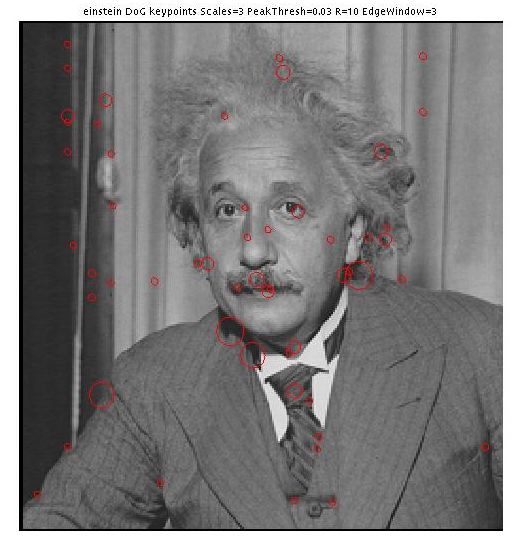 |
  53 points:
   x coord   y coord    sigma
   ----------------------------
   24.0000   52.0000   10.1594
   48.0000   52.0000   10.1594
   96.0000  218.0000   10.1594
  102.0000   52.0000   10.1594
  104.0000   84.0000   10.1594
  132.0000   52.0000   10.1594
  134.0000   98.0000   10.1594
  186.0000  100.0000   10.1594
  188.0000  240.0000   10.1594
  208.0000  390.0000   10.1594
  210.0000  264.0000   10.1594
  218.0000  242.0000   10.1594
  226.0000   58.0000   10.1594
  264.0000   98.0000   10.1594
  270.0000  266.0000   10.1594
  334.0000  286.0000   10.1594
  382.0000  308.0000   10.1594
  418.0000  318.0000   10.1594
  428.0000   52.0000   10.1594
  430.0000  316.0000   10.1594
  464.0000  150.0000   10.1594
  476.0000   20.0000   10.1594
  482.0000  292.0000   10.1594
  484.0000  332.0000   10.1594
   36.0000  428.0000   12.8000
   38.0000  276.0000   12.8000
   92.0000  428.0000   12.8000
  218.0000  370.0000   12.8000
|
einstein.jpg - results of running einstein with PeakThresh=0.08, InitSigma=1.6, Slices=3, R=10 for 3 octaves:
 |
  15 points:
  x coord   y coord    sigma
  ----------------------------
  194.0000  226.0000   10.1594
  224.0000  180.0000   10.1594
  270.0000  266.0000   10.1594
  272.0000  286.0000   10.1594
  334.0000  286.0000   10.1594
  382.0000  308.0000   10.1594
  476.0000   20.0000   10.1594
  192.0000  364.0000   12.8000
  252.0000  350.0000   12.8000
  268.0000  232.0000   12.8000
  362.0000  276.0000   12.8000
  272.0000  268.0000   40.6375
  328.0000  292.0000   40.6375
  256.0000  344.0000   51.2000
  308.0000  220.0000   51.2000
  220.0000  330.0000   12.8000
  244.0000  190.0000   12.8000
  252.0000  350.0000   12.8000
  254.0000   78.0000   12.8000
  260.0000  406.0000   12.8000
  262.0000  144.0000   12.8000
|
  x coord   y coord    sigma
  ----------------------------
  268.0000  232.0000   12.8000
  278.0000   78.0000   12.8000
  428.0000  494.0000   12.8000
   80.0000   92.0000   40.6375
   96.0000   52.0000   40.6375
  192.0000  296.0000   40.6375
  220.0000  388.0000   40.6375
  244.0000  200.0000   40.6375
  272.0000  264.0000   40.6375
  328.0000  292.0000   40.6375
   52.0000  280.0000   51.2000
  132.0000  384.0000   51.2000
  256.0000  344.0000   51.2000
  260.0000  252.0000   51.2000
  372.0000  292.0000   51.2000
  336.0000  248.0000  162.5499
  376.0000   88.0000  162.5499
  256.0000  360.0000  204.8000
  312.0000  224.0000  204.8000
|
problem one - part two b)
einstein05:
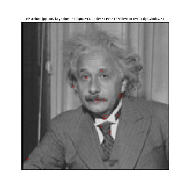 |
  12 points:
  x coord   y coord    sigma
  ----------------------------
  194.0000  226.0000   10.1594
  224.0000  180.0000   10.1594
  272.0000  286.0000   10.1594
  334.0000  286.0000   10.1594
  382.0000  308.0000   10.1594
  474.0000   22.0000   10.1594
  170.0000  278.0000   12.8000
  324.0000  334.0000   12.8000
  362.0000  276.0000   12.8000
  272.0000  264.0000   40.6375
  328.0000  292.0000   40.6375
  256.0000  344.0000   51.2000
|
einstein06.jpg:
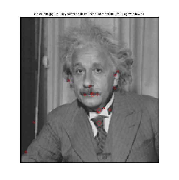 |
  15 points:
  x coord   y coord    sigma
  ----------------------------
  206.0000  352.0000   10.1594
  224.0000  180.0000   10.1594
  270.0000  266.0000   10.1594
  272.0000  286.0000   10.1594
  274.0000  240.0000   10.1594
  320.0000  310.0000   10.1594
  334.0000  288.0000   10.1594
  370.0000   52.0000   10.1594
  474.0000   22.0000   10.1594
  192.0000  362.0000   12.8000
  244.0000  258.0000   12.8000
  250.0000  350.0000   12.8000
  326.0000  332.0000   12.8000
  272.0000  268.0000   40.6375
  328.0000  292.0000   40.6375
  372.0000  292.0000   51.2000
|
einstein07.jpg
 |
  15 points:
  x coord   y coord    sigma
  ----------------------------
  194.0000  226.0000   10.1594
  200.0000  184.0000   10.1594
  206.0000  352.0000   10.1594
  224.0000  180.0000   10.1594
  334.0000  286.0000   10.1594
  382.0000  308.0000   10.1594
  476.0000   20.0000   10.1594
  192.0000  364.0000   12.8000
  268.0000  232.0000   12.8000
  324.0000  334.0000   12.8000
  362.0000  276.0000   12.8000
  416.0000  290.0000   12.8000
  272.0000  264.0000   40.6375
  328.0000  292.0000   40.6375
  256.0000  344.0000   51.2000
|
einstein08.jpg
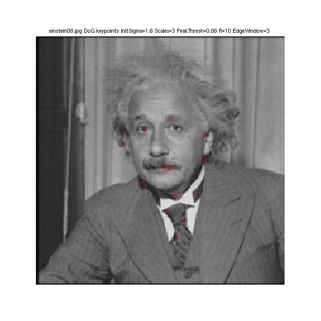 |
  16 points:
  x coord   y coord    sigma
  ----------------------------
  194.0000  226.0000   10.1594
  200.0000  184.0000   10.1594
  206.0000  352.0000   10.1594
  224.0000  180.0000   10.1594
  272.0000  286.0000   10.1594
  274.0000  276.0000   10.1594
  334.0000  286.0000   10.1594
  382.0000  308.0000   10.1594
  170.0000  278.0000   12.8000
  326.0000  334.0000   12.8000
  362.0000  276.0000   12.8000
  416.0000  290.0000   12.8000
  272.0000  268.0000   40.6375
  328.0000  292.0000   40.6375
  256.0000  344.0000   51.2000
  308.0000  220.0000   51.2000
|
einstein-09.jpg
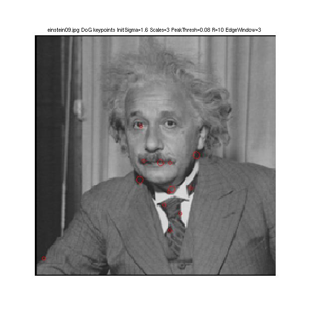 |
  13 points:
  x coord   y coord    sigma
  ----------------------------
  194.0000  226.0000   10.1594
  272.0000  288.0000   10.1594
  334.0000  286.0000   10.1594
  380.0000  310.0000   10.1594
  476.0000   20.0000   10.1594
  268.0000  232.0000   12.8000
  326.0000  332.0000   12.8000
  362.0000  276.0000   12.8000
  416.0000  288.0000   12.8000
  272.0000  268.0000   40.6375
  328.0000  292.0000   40.6375
  256.0000  344.0000   51.2000
  308.0000  224.0000   51.2000
|
problem one part two c)
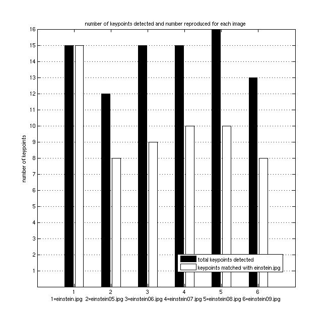
problem one part two d)
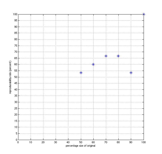
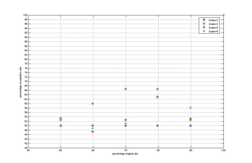
The following is a plot of just the recognition rates for
keypoints when the number of intermediate scales [2, 3, 4, 5],
as a function of how large the image is (ie, which einstein we chose).
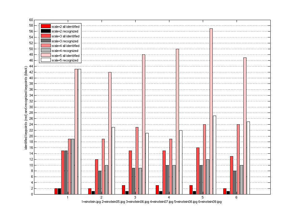
The following is a plot comparing the number of keypoints found when the
number of scales is set to each of 2, 3, 4 and 5 verus the number later
identified.
problem two
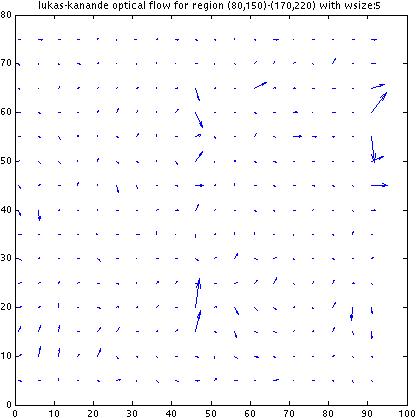
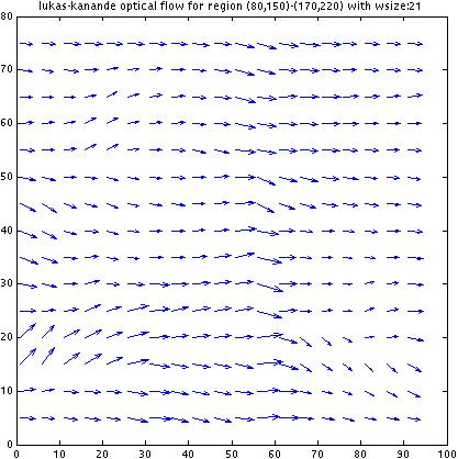
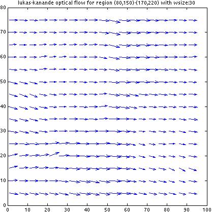
lukas-kanande optical flow tracker
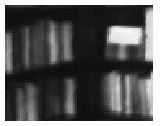
source regions:
patch 0:
 |
patch 1:
 |
%% function [dx,dy] = lucaskanade(I1,I2,xl,yt,xr,yb,wsize)
%% computes the optical flow over an image region (xl->xr, yt->yb)
%% from I1 to I2 using a patch of size wsize by solving the Lucas Kanade
%% BCCE (brightness constant constraint equation)

function [lkdx,lkdy] = lucaskanade(I1,I2,xl,yt,xr,yb,wsize)

function W = getWindow(image,x,y)
   %% returns window of image centered at (x,y) of size
   %% (wsize)x(wsize)
   half = floor(wsize/2);
   W = image([y-half:y+half],[x-half:x+half]);
end;

function [bcce_dx,bcce_dy] = BCCE(x,y)
    patch_dx = getWindow(i1dx,x,y);
    patch_dy = getWindow(i1dy,x,y);
    patch_dt = getWindow(dI,x,y);

    ix2 = sum(sum(patch_dx.^2));
    iy2 = sum(sum(patch_dy.^2));
    ixiy = sum(sum(patch_dx.*patch_dy));
    A = [ix2 ixiy; ixiy iy2];

    ixit = sum(sum(patch_dx.*patch_dt));
    iyit = sum(sum(patch_dy.*patch_dt));
    b = -1 * [ixit; iyit];

    u = pinv(A)*b; % A\b;
    bcce_dx = u(1); bcce_dy = u(2);
end;

i1 = I1;
[i1dx i1dy] = gradient(i1);

% approximate the temporal gradient by a blurred difference
% between the two images
dI = blurGauss(I2,2.0)-blurGauss(I1,2.0);

lkdx = []; lkdy = [];

for xi=xl:xr,
  for yi=yt:yb,
    [dix,diy]= BCCE(xi,yi);
    lkdx(yi-yt+1,xi-xl+1)= dix;   lkdy(yi-yt+1,xi-xl+1)= diy;
  end;
end;

%% kill nans
lkdx(isnan(lkdx)) = 0;
lkdy(isnan(lkdy)) = 0;

end
results:
parts b and c)
Although from visual inspection from the images it seems that
the optical flow should be the same over the whole region (the
two images are basically the result of a very slight camera
displacement to the righttos) looking at the results we see
that the conclusions that our lukas-kanande algorithm draws
are quite different.
For small window sizes, w, the algorithm is very sensitive
to local variations of brightness within the image texture,
and gets thrown off by this. In these situations, while
most of the gradients do indicate a general trend in the proper direction, many
display evidence of upwards or downwards displacmeent.
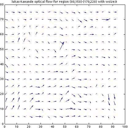
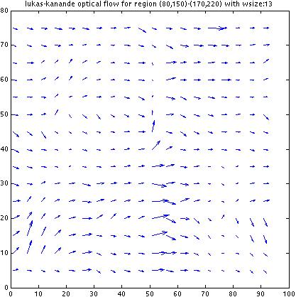
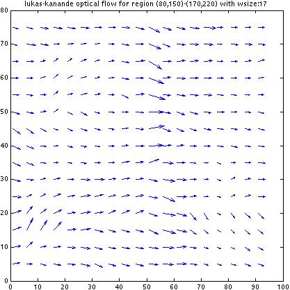
As we increase w, the optical flow vectors start to
stabilize and agree to the "correct solution". which is
fine for this particular image since the optical flow for
the whole image is the same. However, since this algorithm
computes flow within a window as if the flow at every location
within the whole patch is the same, increasing w will be
deterimental for an image where there are actual local variations
of flow. I am not sure how to get around this; that is,
how to compute flow fields for highly location-sensitive
optical flows against richly textured backgrounds.