Whereas Bayesian networks are directed graphical models, random fields (aka Markov networks) are
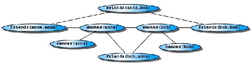
undirected graphical models defining the joint distribution of some set of random variables. As an example
consider the following smoker random field inspired by Richardson and Domingos:
In recent years, CRFs have been most often used for labeling and segmenting structured data,
such as sequences, trees and lattices. Here, we will focus on so-called linear-chain CRFs.
Let G be an undirected graphical model over sets of random variables
X and Y, where X = < xi > and Y = < yi >
are sequences of symbols, so that Y is a labeling of an the observed input sequence X.
Then, linear-chain CRFs define the conditional probability of a state sequence given the observed
sequence as
P(Y|X) = (1/Z(X)) * exp( sum_t pi(t,yt,X) + pi(t-1,yt-1,yt,X) ), |
where pi(t,yt,X) and pi(t-1,yt-1,yt,X) are potential functions and Z(X) is a normalization factor over all state sequences X. A potential function is a real-valued function that captures the degree to which the assignment yt to the output variable fits the transition from yt-1 and X. Due to the global normalization by Z(X), each potential has an influence on the overall probability.
To apply CRFs to a labeling problems, one must choose a representation for the
potentials. Typically, it is assumed that the potentials factorize according to a
set of features {gk} resp. {fk}, which are given and fixed, so that
pi(t,yt,X) = Sum vk * gk(yt,X) resp. pi(t,yt,X) = Sum wk * fk(t-1,yt-1,yt,X). |
In other words, the potential are linear combinations of the input features. Consequently, the model parameters are now a set of real-valued weights, one weight for each feature. In linear-chain CRFs, a first-order Markov assumption is made on the hidden variables. Note that feature functions can be arbitrary such as a binary test that has value 1 if and only if yt is subsumed by some logical formula.