Hello, Halide!
Halide employs a static metaprogramming model similar to Tensorflow or Terra. We write C++ or Python programs that construct Halide functions that describe the algorithm. Halide then transforms these functions into lower-level code based on the schedules. This has two benefits. First, it allows the compiler frontend to be embedded in a popular language. This makes interaction of Halide with these languages easier, and allows metaprogramming Halide functions using the host language. Second, in contrast to interpreting a dynamic computation graph, the static model enables Halide to generate more efficient code by employing compiler optimizations ahead of the time. This is important for the scheduling part of Halide to have effect.
Following is a Halide program that loads an image, makes it two times brighter, and save to an image file.
// To compile & run on Linux
// g++ hello_halide.cpp -g -I /path/to/halide/distrib/include -I /path/to/halide/distrib/tools -L /path/to/halide/distrib/bin -lHalide `libpng-config --cflags --ldflags` -ljpeg -lpthread -ldl -o hello_halide -std=c++11
// LD_LIBRARY_PATH=/path/to/halide/distrib/bin ./hello_halide
// MacOS
// g++ hello_halide.cpp -g -I /path/to/halide/distrib/include -I /path/to/halide/distrib/tools -L /path/to/halide/distrib/bin -lHalide `libpng-config --cflags --ldflags` -ljpeg -o hello_halide -std=c++11
// DYLD_LIBRARY_PATH=/path/to/halide/distrib/bin ./hello_halide

#include <Halide.h>
#include <halide_image_io.h>

using namespace Halide;
using namespace Halide::Tools;

int main() {
    // Constructing Halide functions statically.
    //
    ImageParam input(Float(32), 3);
    Func f("f");
    Var x("x"), y("y"), c("c");
    // Double the values and clamp them by 1.
    f(x, y, c) = min(2 * input(x, y, c), 1.f);

    // Actually compiling/executing the Halide functions.
    //
    // Setup the input by loading an image.
    Buffer<float> input_buffer = load_and_convert_image("images/rgb.png");
    input.set(input_buffer);
    // Process the input by calling f.realize
    Buffer<float> output_buffer = f.realize(
        input_buffer.width(), input_buffer.height(), input_buffer.channels());
    // Save the image to a file.
    convert_and_save_image(output_buffer, "output.png");
}
import halide as hl
import imageio
import numpy as np

# Constructing Halide functions statically.
input = hl.ImageParam(hl.Float(32), 3)
f = hl.Func('f')
x, y, c = hl.Var('x'), hl.Var('y'), hl.Var('c')
# Double the values and clamp them by 1.
f[x, y, c] = hl.min(2 * input[x, y, c], 1.0)

# Actually compiling/executing the Halide functions.
#
# Setup the input by loading an image (Halide assumes Fortran ordering).
img = hl.Buffer(np.asfortranarray(imageio.imread('images/rgb.png').astype(np.float32) / 255.0))
input.set(img)
# Process the input by calling f.realize
output = f.realize(img.width(), img.height(), img.channels())
# Save the image to a file by converting to a numpy array.
output = np.array(output)
imageio.imsave('output.png', (output * 255.0).astype(np.uint8))
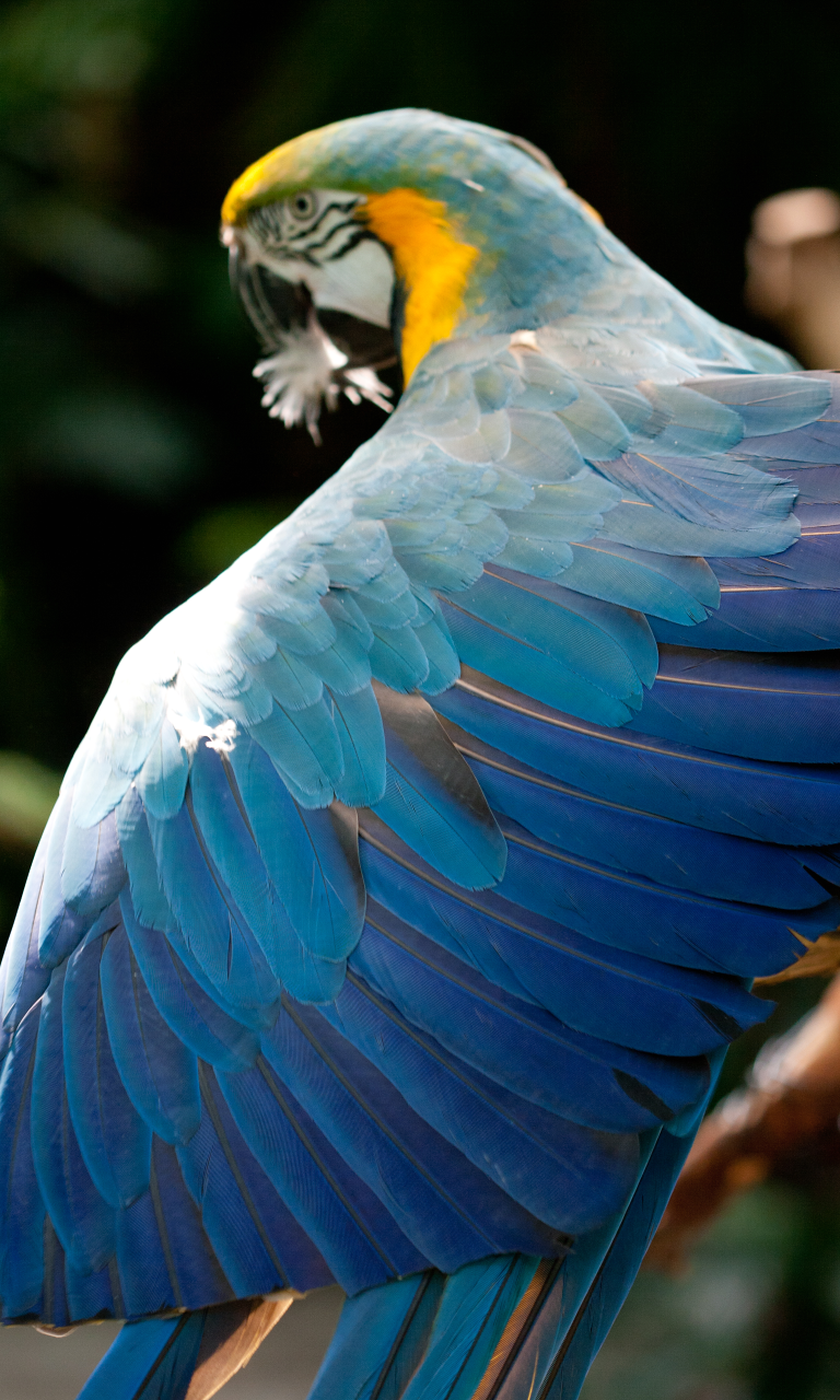
This is our input:
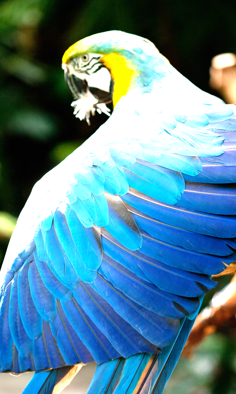
And this is our output:
We will explain the code line by line.
To use Halide in our program, we need to include the Halide header in C++ or import the Halide module in Python:
#include <Halide.h>
#include <halide_image_io.h>

using namespace Halide;
using namespace Halide::Tools; // For loading/saving images
import halide as hl
Halide’s input can be represented with an ImageParam, which is a multi-dimensional array.
The first arugment describes the type of the array, and the second argument describes the dimensionality.
ImageParam input(Float(32), 3);
# Construct an ImageParam with 3 dimensions
input = hl.ImageParam(hl.Float(32), 3)
Remember that we are metaprogramming Halide code. The input does not have an actual value yet. We will define it’s content when we actually execute the Halide program.
Computations are defined in Halide functions.
The following code declares a Halide function f, that does not has a definition yet:
Func f("f");
f = hl.Func('f')
The constructor of Func takes an optional name argument that is useful for
debugging and pretty printing.
Each Halide function describes an infinite multi-dimensional domain of values. This means that, when accessing a Halide function, it always returns some value or triggers an out-of-bound assertion. This has the benefit of memory safety – Halide guarantees that we can never have buffer overrun issues that cause segmentation faults. This relieves the programmers from having to worry about the boundaries of a computation.
To describe the multi-dimensional domain, we need to name the coordinates.
Var is designed for this:
Var x("x"), y("y"), c("c");
x, y, c = hl.Var('x'), hl.Var('y'), hl.Var('c')
Once we have Func and Var declared, we are ready to describe our computation:
// Double the values and clamp them by 1.
f(x, y, c) = min(2 * input(x, y, c), 1.f);
# Double the values and clamp them by 1.
f[x, y, c] = hl.min(2 * input[x, y, c], 1.0)
Again, keep in mind that we are metaprogramming Halide functions – at this point
there is no f computed. We don’t even have our input contents yet!
Note
Apart from arrays, we can also define 0-dimensional Halide functions to represent scalars:
Func g("g");
g() = 5.0f;
g = hl.Func('g');
g[()] = hl.f32(5.0)
Now we finished defining our Halide functions, we want to use it for computing something.
First we need to setup our inputs. They are represented by Halide Buffer s.
Unlike Halide Func s, they are multidimensional arrays that actually store values.
Buffer<float> input_buffer = load_and_convert_image("images/rgb.png");
input_buffer = hl.Buffer(np.asfortranarray(imageio.imread('images/rgb.png').astype(np.float32) / 255.0))
Halide’s Python frontend works seamlessly with numpy. However, note that
Halide Buffer assumes Fortran ordering (dimensions to the left correspond to
innermost storage), so we want to use np.asfortranarray to convert our numpy arrays.
Next we set the content of the input to the buffers we just created.
input.set(input_buffer);
input.set(input_buffer)
Now, to actually compute a window of f, we need to call f.realize. This
generates a Buffer that has a finite extent and actual values inside:
// Process the input by calling f.realize
Buffer<float> output_buffer = f.realize(
    input_buffer.width(), input_buffer.height(), input_buffer.channels());
# Process the input by calling f.realize
output = f.realize(input_buffer.width(), input_buffer.height(), input_buffer.channels())
Finally we save the output image to a file, and we’re done!
// Save the image to a file.
convert_and_save_image(output_buffer, "output.png");
# Save the image to a file by converting to a numpy array.
output = np.array(output)
imageio.imsave('output.png', (output * 255.0).astype(np.uint8))
Note
We can read/write Halide Buffer s using operator() in C++ and __getitem__ in Python.
Buffer<float> b(100);
for (int i = 0; i < 100; i++) {
    b(i) = float(i);
}
b = hl.Buffer(hl.Float(32), 100);
for i in range(100):
    b[i] = float(i)
Note
We can create a 0-dimensional Buffer using make_scalar().
Buffer<float> b = Buffer<float>::make_scalar();
b() = 1.f;
b = hl.Buffer.make_scalar(hl.Float(32))
b[()] = 1.0
Note
We can use Halide Buffer s as if they are ImageParam.
Buffer<int> b(3);
Func f("f");
Var x("x");
f(x) = b(x);

// fill in b
b(0) = 1; b(1) = 2; b(2) = 5;
// realize f
f.realize(b.width());
b = hl.Buffer(hl.Int(32), 3)
f = hl.Func("f")
x = hl.Var("x")
f[x] = b[x]

# fill in b
b[0] = 1; b[1] = 2; b[2] = 5
# realize f
f.realize(b.width())
In the next tutorial we will talk about how to write more complex Halide algorithms using examples.