IEEE Conference on Computer Vision and Pattern Recognition 2010
Exploring Features in a Bayesian Framework for Material Recognition
Ce Liu1,3 Lavanya Sharan2 Edward H. Adelson3 Ruth Rosenholtz3
1Microsoft Research New England 2Disney Research Pittsburgh 3Massachusetts Institute of Techonolgy
|
Introduction
We are interested in identifying the material category, e.g. glass, metal, fabric, plastic or wood, from a single image of surface. For this purpose, we employed the Flickr Material Database (FMD) [3], which consists of 10 common material categories and 100 diverse images per category. In this paper, we formulate the material recognition problem as being able to recognize a given input image (from the database) as belonging to one of these 10 material categories.
|
||||||||||||||||||||||||||||||||||||
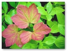
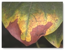
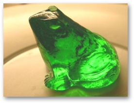
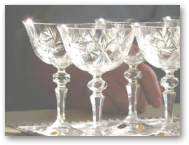
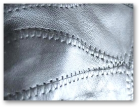
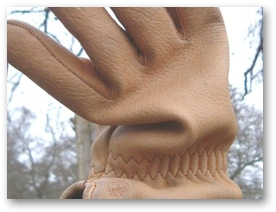
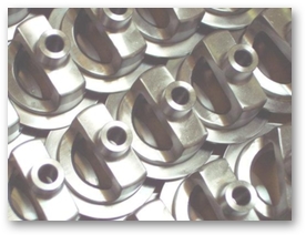
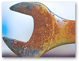
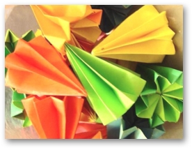

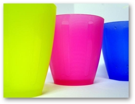

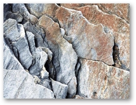

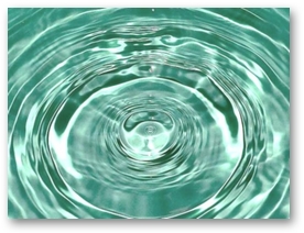
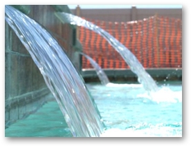
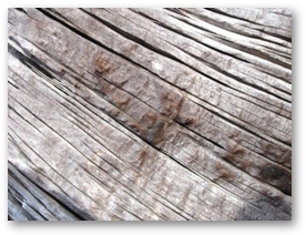
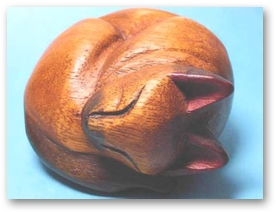
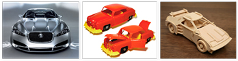
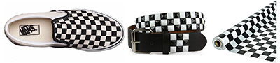
Material recognition is quite different from traditional shape-based object recognition as well as texture recognition. Consider these illustrations:
|
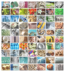
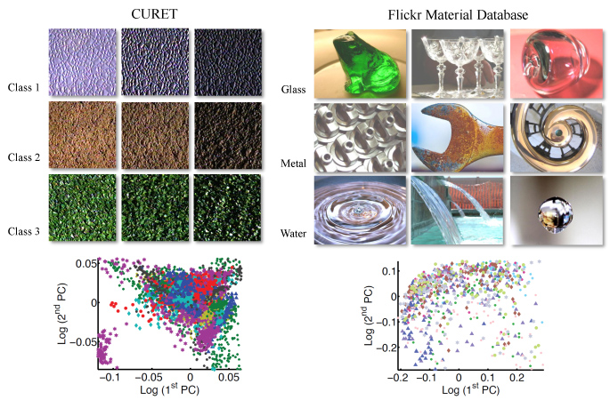
The sheer diversity in material appearance makes material recognition a challenging problem. Instances from a single material category can span a range of object categories, shapes, colors, textures, lighting and imaging conditions. Previous work on this topic has focused on recognizing instances from the CURET database [4] that consists of 61 different texture samples, under 205 viewing and lighting conditions. Although >95% recognition rates have been reported on CURET, we believe that the intra-class variation in appearance in the CURET database is too limited to capture the complexity of real world materials, as shown in Fig 4.
|
Features for material recognition
It is essential to identify reliable features for material recognition. Perhaps, a single feature is insufficient for material recognition. Our strategy has been to try a variety of low-level and middle-level features and to combine them for recognition.
From a rendering point of view, once the camera and the object are fixed, the image of the object can be determined by (i) the BRDF of the surface, (ii) surface structures, (iii) object shape and (iv) environment lighting. Although it is nearly impossible to infer each of these factors from a single image, we can measure some image features that are correlated with these factors.
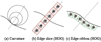
Fig 5. We extract curvature at three scales, edge slice in 6 cells and edge ribbon in 6 cells at edges. |
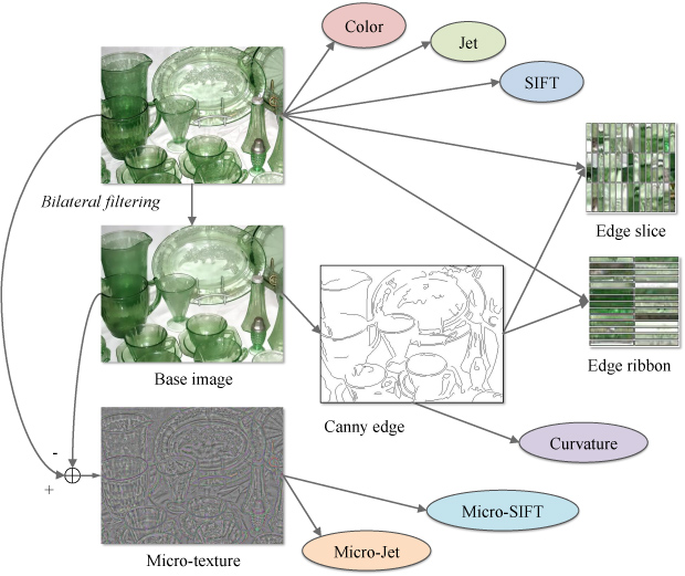
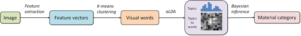
Fig 6. Illustration of how our system generates features for material recognition |
|
|
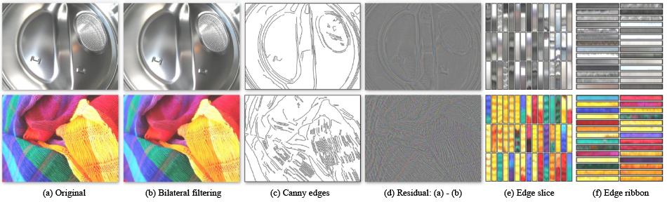
Fig 7. Some features for material recognition. From top to bottom is metal and fabric. For an image (a) we apply bilateral filtering to obtain the base image (b). We run Canny edge detector on the base image and obtain edge maps (c). Curvatures of the edges are extracted as features. Subtracting (b) from (a), we get the residual image (d) that shows micro structures of the material. We extract micro-jet and micro-SIFT features on (d) to characterize material micro-surface structure. In (e), we also show some random samples of edge slices along the normal directions of the Canny edges. These samples reveal lighting-dependent features such as specular highlights. The edge ribbon samples are shown in (f). Arrays of HOG's [7] are extracted from (e) and (f) to form edge-slice and edge-ribbon features. |
Augmented Latent Dirichlet Allocation (aLDA)
|
| Figure 8. The flowchart of our system. We used the bag of words model to represent images and learned a genereative model for each class for recognition. |
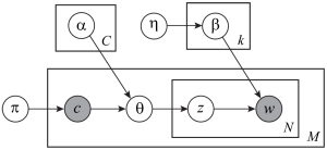
After the features are quantized into visual words, each image is treated as a document model (bag of words). We use latent Dirichlet allocation (LDA) to model the distribution of visual words for each category with following extensions (please refer to the paper for the details of the algorithm):
|
Fig 9. The graphical model of LDA [1]. Notice that our categorization shares both the topics and codewords. |
Experimental results
|
We used the Flickr Material Database for all the experiments. There are 10 classes in FMD, and each class contains 100 images, 50 of which are close-up views and the rest 50 are of views at object-scale. There is a binary, human labeled mask associated with each image describing the location of the object. Only the pixels inside the binary mask are considered for material recognition. For each category, we randomly chose 50 images for training and 50 images for test. All the results are repoted based on the same split of training and test. We extract features for each image according to Fig. 6. Mindful of computational costs, we sample color, jet, SIFT, micro-jet and micro-SIFT on a coarse grid (every 5th pixel in both horizontal and vertical directions). Because there are fewer pixels in edge maps, we sample every other edge pixel for curvature, edge-slice and edge-ribbon. Once features are extracted, they are clustered separately using k-means according to the number of clusters in Table 1. |
Table 1. The dimension, number of clusters and average number per image for each feature. |
After forming the dictionaries for each feature, we run the aLDA algorithm to select features incrementally. In the LDA learning step, we vary the number of topics from 50 to 250 with step size 50 and pick the best one. The learning procedure is shown in Fig 10, where for each material category we plot the training rate on the left in a darker color and the test rate on the right in a lighter color. In the beginning, the system tries every single feature and discovers that amongst all the features, SIFT produces the highest evaluation rate. In the next iteration, the system picks up color from the reaiming features, and then edge-slice. Including more features causes the performance to drop and the algorithm stops. For the final feature set "color + SIFT + edge-slice", the training rate is 49.4% and the test rate is 44.6%. The recognition rate of random guess is 10%.
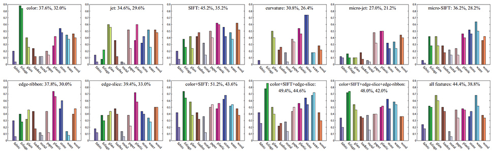 |
| Fig 10. The per-class recognition rate (both training and test) with different sets of features for FMD. In each plot, the left, darker bar means training, the right, lighter bar means test. For the two numbers right after the feature set label are the training and test recognition rate. For example, "color: 37.6%, 32.0%" means that the training rate is 37.6% and the test rate is 32.0%. Our aLDA algorithm finds "color + SIFT + edge-slice" to be the optimal feature set on the Flickr Materials Database. |
For comparison, we implemented and tested Varma-Zisserman's (VZ) algorithm [4] on FMD. The VZ algorithm clusters 5x5 pixel gray-scale patches as codewords, obtains a histogram of the codewords for each image, and performs recognition using a nearest neighbor classifier. We ran VZ algorithm on FMD and obtained test rate 23.8% (ours is 44.6%). As the VZ system uses features tailored for the CURET database (5x5 patches), we ran VZ's algorithm using our features on FMD. The results of running VZ's system on exactly the same fature sets as in Fig 10 are listed in Fig 11. Since VZ uses a nearest neighbor classifer, it is meaningless to report the training rate as it is always 100%, so we only report the test rate. The VZ system running on SIFT feature has test rate of 31.8%, close to our system using SIFT alone (35.3%). However, combining features under the VZ's framework only slightly increases the performance to a maximum of 37.4%. Clearly, the aLDA framework contributes to the boost in performance from 37.4% to 44.6%.
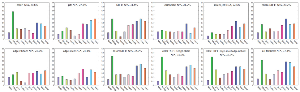 |
| Fig 11. For comparison, we run Varma-Zisserman's system [4] (nearest neighbor classifiers using histograms of visual words) on our feature sets. Because of the nearest neighbor classifier, the training rate is always 100%, so we simply put it as N/A. |
 |
 |
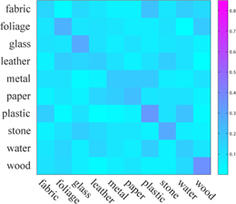 |
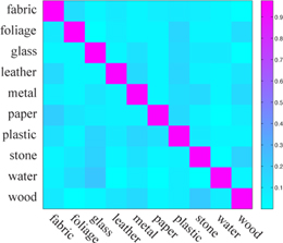
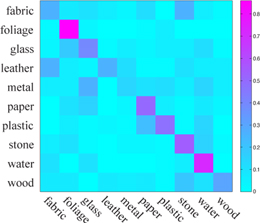
| (a) 500 Mechanical Turkers (avg: 92.3%) | (b) Our system (avg: 44.6%) | (c) Varma-Zisserman [4] (avg: 23.8%) |
| Fig 12. Confusion matrices of human and material recognition. (a) We obtained the human recognition rate on FMD through conducting an experiment on Mechanical Turk by asking 500 individuals and obtaining the average. (b) The confusion matrix of our material recognition system using "color + SIFT + edge-slice" feature set. (c) The confusion matrix of directly running Varma-Zisserman's system on FMD. |
|
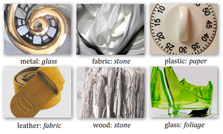
Some misclassification examples of our system are shown on the right. Label “metal: glass” means a metal material is misclassified as glass. Some of these examples can be ambiguous to humans. |
 |
Conclusion
To conclude, we have presented a set of features and a Bayesian computational framework for material category recognition. Our features were chosen to capture various aspects of material appearance in the real world. An augmented LDA (aLDA) framework was designed to select an optimal set of features by maximizing the recognition rate on the training set. We have demonstrated a significant improvement in performance when using our system over the state of the art on the challenging Flickr Materials Database. We have also analyzed the contribution of each feature in our system to the performance gain. Our feature set and computational framework constitute the first attempt at recognizing high-level material categories "in the wild''.
References
| [1] | D. M. Blei, A. Y. Ng, and M. I. Jordan. Latent Dirichlet Allocation. Journal of Machine Learning Research, (3):993– 1022, 2003. |
| [2] | C. Liu, L. Sharan, E. H. Adelson and R. Rosenholtz. Exploring features in a Bayesian framework for material recognition. To appear at CVPR 2010. |
| [3] | L. Sharan, R. Rosenholtz, and E. Adelson. Material perception: What can you see in a brief glance? [Abstract]. Journal of Vision, 9(8):784, 2009. |
| [4] | M. Varma and A. Zisserman. A statistical approach to material classification using image patch exemplars. TPAMI,31(11):2032–2047, 2009. |
Last update: June, 2010