Learning Inhomogeneous Gibbs Models (IGM)

Ce Liu*   Heung-Yeung Shum^†   Song Chun Zhu^¶

*Massachusetts Institute of Technology (the work was done when I interned at MSRA)

^†Microsoft Research Asia

^¶University of California, Los Angeles

International Conference on Computer Vision (ICCV), 2001

Download [pdf], [ppt] (presented at AI Lab, MIT)

What

In this paper we present an inhomogeneous Gibbs model (IGM) to learn high-dimensional distributions for inhomogeneous visual patterns. The IGM has the following properties. First, IGM employs a number of linear features (not necessarily orthogonal) and corresponding discrete histograms from the observed samples as robust statistics to describe the distribution. Second, an inhomogeneous Gibbs distribution is derived based on the maximum entropy principle. The Gibbs potential functions with respect to the linear features are trained to match the observed histograms using Monte Carlo sampling. Third, the linear features are incrementally introduced into the IGM based on the minimum entropy principle. Each new feature, called a KL feature is learnt by maximizing the approximate information gain, or the KL divergence introduced by the new feature while keeping the parameters of the previous model unchanged. Unlike previous minimax entropy models, IGM does not select features from a pre-defined pool of candidates, but automatically learns in the form of linear features.

Why

1. Non-Gaussianity. What is the form of the underlying distribution? Is there any basic principle we can follow to find the form? Not surprisingly, most natural data are non-Gaussian distributed.

2. Small samples vs. high dimensions. Usually we only have sparse data in the high-dimensional space. For instance, we wish to learn the distribution for 32x48 (1536 dimensions) face patches from 3000 sample images. Each dimension gets on average fewer than two sample images, yet collecting 3000 sample images takes significant effort in practice. What kind of features are suitable to capture the characteristics of the sparse data, so that the learnt model can generalize very well?

3. Robust parameter estimation. There are always parameters for any form of distributions. Could we reliably estimate the global optimal parameters, without being stuck at a local optimum? Meanwhile, overfitting should be avoided to ensure good generalization ability.

In this paper we propose a statistical model to tackle the above challenges inspired by [3].

How

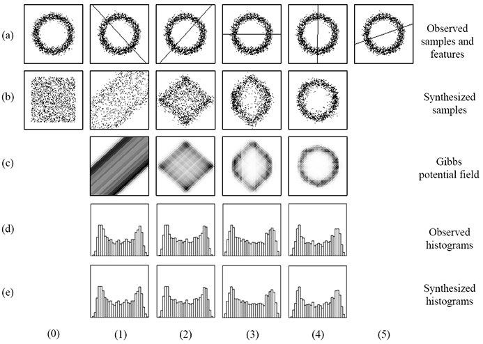
The key idea is to reconstruct the joint pdf in high-dimensional space using the marginal distributions on linear features. Please refer to the paper and slides for detailed math and computation. Here we use a toy example to explain how IGM works, as shown below. A set of independent samples is drawn from this distribution, as shown in row (a), column (0) (denoted as (a0) for simplicity). Before any features are selected, the potential form of the Gibbs distribution is zero and thus the synthesized samples are uniformly distributed as shown in (b0). After comparing the observed (a0) and synthesized samples (b0), the first feature is pursued by maximizing the projected KL divergence. This feature is shown in (a1) along with all observed samples. Samples drawn from the resulting IGM (with the learnt feature) are shown in (b1). The corresponding Gibbs potential field is shown in (c1). The darker a pixel is, the smaller Gibbs potential it represents. The synthesized samples (b1) can be compared with the observed (a0) to pursue the second feature which is shown in (a2). A new IGM is learnt from these two features, and the samples synthesized from this IGM are shown in (b2), with corresponding Gibbs potential field in (c2). This process continues until the information gain (KL divergence) by adding the 5th feature. The Gibbs model with these four learnt features can adequately describe the underlying distribution, as we observe that the synthesized sample set (b4) is very similar to the observed (a0). This is also demonstrated by the perfect match between the histograms for both the observed and synthesized samples with these two features, as shown in row (d) and (e). The Gibbs sampling process can be sped up by importance sampling [2].

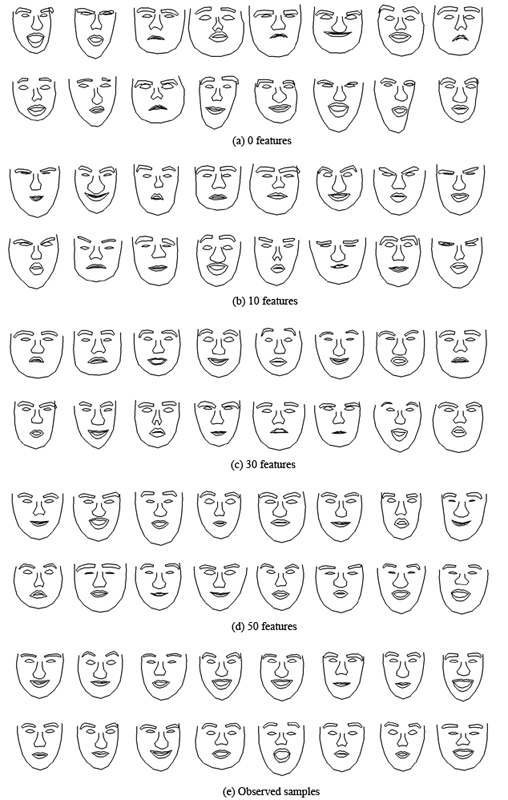
(Note that the results reported here are slightly different from the original paper because we trained on a different data set.) In our experiment we collected 720 face images and manually labelled 83 landmarks. First we use PCA to reduce the original high-dimensional (166) problem to a lower 33-dimensional subspace. Some typical training faces from our 720 training examples are shown in the bottom-left figure (row (e)). 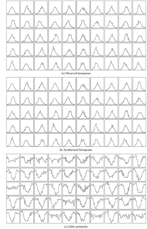At each parameter learning step, we have drawn 40, 000 samples by the Gibbs sampler. The results synthesized by the model with 0, 10, 30 and 50 features are shown in the left. The model found that 50 features are enough to capture the statistics of the observed data. The observed and synthesized histograms, along with the learnt Gibbs potentials, are plotted in the bottom-right figure. Note that most of these potentials do not have a quadratic form. This implies that it is inappropriate to assume a Gaussian model for faces.