This file documents FreeSnell 1c4 (released January 2024), a simulator for thin-film optics.
Copyright © 2003, 2004, 2007, 2009, 2010 Aubrey Jaffer
Permission is granted to make and distribute verbatim copies of this manual provided the copyright notice and this permission notice are preserved on all copies.
Permission is granted to copy and distribute modified versions of this manual under the conditions for verbatim copying, provided that the entire resulting derived work is distributed under the terms of a permission notice identical to this one.
Permission is granted to copy and distribute translations of this manual into another language, under the above conditions for modified versions, except that this permission notice may be stated in a translation approved by the author.
Next: Optical Properties of Materials, Previous: FreeSnell, Up: FreeSnell [Contents][Index]
Some wondrous optical technology can result from depositing coatings less than a few micrometers thick on glass, plastic, and other surfaces. These coatings are used to enhance the reflectivity of astronomical mirrors or diminish the reflections from visual displays and lenses; they can improve the efficiency of window glass and solar cells.
FreeSnell computes these effects for parallel layers of dielectric and conductive materials.
Next: Theory of Operation, Previous: Overview, Up: Overview [Contents][Index]
I couldn’t find a free implementation of thin-film optical calculations I needed for a project. So I rolled my own.
The first versions were based on webpages [NCSU] and [Nave], but differences in signs and conventions of the complex index of refraction caused havoc with metallic layers. [Sernelius] has a comprehensive treatment with signs consistent from start to finish. The current version is based on that.
The properties of granular films are taken from [Heavens] discussion of Maxwell Garnett theory. [Granfilm] computes properties of granular films with great sophistication, but appears to require a PhD in physics in order to use it.
Optics is wavelength based; so this package is also. These routines work out the complex voltages in the forward and reverse directions to find the transmitted and reflected amplitudes. This works only for intensities where the layers act linearly (superposition).
Each layer 0:n has an index of refraction and height. Because the P and S polarizations are independent, they are calculated separately. The square of the absolute value of computed field values expressing power ratios are the returned quantities.
Next: Wrinkles, Previous: Background, Up: Overview [Contents][Index]
The effects of coatings on light are determined by Snell’s law and Fresnel’s equations, which model the light’s electric and magnetic fields.
Taking the Laplace-transform of the differential equations relating the fields at the surface of each parallel layer of materials yields algebraic equations relating the indexes-of-refraction and the (complex) attenuation and phase as functions of wavelength.
These algebraic equations can be organized into products of 2x2 matrices and 2-vectors. The 2-vectors represent the Laplace transforms of the forward and reverse radiation. Each interface between adjacent materials corresponds to a 2x2 matrix.
The product of the chain of 2x2 matrices produces a single 2x2 matrix expressing the transmittance and reflectance of the layered stack as a whole, solving the system of equations.
This method is not unique to thin-film optics; it is essentially the same as the 2-port method for analysis of linear electrical circuits.
Next: Bibliography, Previous: Theory of Operation, Up: Overview [Contents][Index]
Because these optical systems are passive and linear, the attenuation of radiation passing through in one direction must be the same as the attenuation of radiation passing through in the opposite direction.
Radiation that is not transmitted through the stack must be either absorbed or reflected. The absorption at the top is not necessarily the same as the absorption at the bottom.
Rays impinging on the stack with non-normal incidence will leave the stack with non-normal incidence; the angles being identical if the indexes of refraction of the top and bottom materials are identical.
Rays impinging on the stack with non-normal incidence have different attenuation and reflectance depending on the polarization of the impinging radiation. FreeSnell computes outcomes for both polarizations; and can report these separately or averaged.
Heavens, O. S., “Optical Properties of Thin Solid Films”, ISBN: 0486669246, Dover Pubns, Dec 1991
Bo E. Sernelius,
“Electrodynamics”,
Dept. of Physics and Measurement Technology, Linköping University
http://www.ifm.liu.se/~boser/elma/, especially
“REFLECTION FROM A METALLIC SURFACE”
http://www.ifm.liu.se/~boser/elma/Lect13.pdf
Lide, D.R., Dr. Editor, “CRC Handbook of Chemistry and Physics (3rd Electronic Edition)”, CRC Press, 2000
“Fresnel’s equations” from the chemistry department of
North Carolina State University.
http://web.archive.org/web/20041029131241/http://chsfpc5.chem.ncsu.edu/CH795Z/lecture/lecture8/fresnel/fresnel.html
“Fresnel’s Equations: Reflection and Transmission” by Carl R. Nave,
Department of Physics and Astronomy, Georgia State University.
http://hyperphysics.phy-astr.gsu.edu/hbase/phyopt/freseq.html
J. C. Maxwell Garnett,
“Colours in Metal Glasses and in Metallic Films”,
Phil. Trans. Roy. Soc. London 203A, 385 (1904).
http://rsta.royalsocietypublishing.org/content/203/359-371/385
R. Lazzari and I. Simonsen, “Granfilm: a software for calculating thin-layer dielectric properties and fresnel coefficients”, Thin Solid Films, 419:124, 2002. http://www.insp.jussieu.fr/axe2/Oxydes/GranFilm/GranularFilm.html
Bartl J, Baranek M (2004), “Emissivity of aluminium and its importance for radiometric measurement”, Measurement of Physical Quantities 43:31–36. http://www.measurement.sk/2004/S3/Bartl.pdf
Michael F Modest, “Radiative heat transfer”, second edition, Academic Press 2003
Next: Material Databases, Previous: Overview, Up: FreeSnell [Contents][Index]
The salient optical properties of a material are specified by its complex index of refraction; which differs from the common index of refraction, n, by incorporating the extinction-coefficient, k/n. There are several conventions for the complex index of refraction. The one employed here follows [Sernelius]: (n + k*i).
Dielectric materials typically have k equal to zero and n which varies little with the wavelength of light being analyzed. They are often computed using a single n value.
Metallic or conductive materials have non-zero k and n which can vary wildly with the wavelength of light being analyzed. These values can be determined through a process called ellipsometry.
The Sopra company manufactures spectroscopic ellipsometers. A bundle
of spectra for 278 materials available from
http://www.sopra-sa.com/more/database.asp (Nov 28, 2000) is
included in the FreeSnell distribution database.
The Software Spectra company also distributes the Sopra data, although
rewritten into their proprietary format. But their zip file
http://www.sspectra.com/files/misc/win/SOPRA.EXE
(Macintosh
http://www.sspectra.com/files/misc/mac/Sopra.sea.hqx)
contains
README.TXT identifying the Sopra files.
Included with FreeSnell are the following metal spectra from the CRC Handbook of Chemistry and Physics:
ag.nk: eV       n       k       R(th=0) ; Silver
al.nk: eV       n       k       R(th=0) ; Aluminium
au.nk: eV       n       k       R(th=0) ; Gold, electropolished, Au (110)
cr.nk: eV       n       k       R(th=0) ; Chromium
cu.nk: eV       n       k       R(th=0) ; Copper
fe.nk: eV       n       k       R(th=0) ; Iron
ge.nk: eV       n       k       R(th=0) ; Germanium, single crystal
li.nk: eV       n       k       R(th=0) ; Lithium
ni.nk: eV       n       k       R(th=0) ; Nickel
ta.nk: eV       n       k       R(th=0) ; Tantalum
ti.nk: eV       n       k       R(th=0) ; Titanium (Polycrystalline)
v.nk: eV        n       k       R(th=0) ; Vanadium
w.nk: eV        n       k       R(th=0) ; Tungsten
zn.nk: eV       n       k       R(th=0) ; Zinc, E _|_ to c^28
zn-e.nk: eV     n       k       R(th=0) ; Zinc, E || to c^28
zr.nk: eV       n       k       R(th=0) ; Zirconium (Polycrystalline)
Many of these materials are included in the Sopra bundle; but the CRC data covers a wider wavelength span than the Sopra spectra. Combining the CRC and Sopra files produces wide bandwidth spectra with finer resolution in the visible and near-infrared bands.
Previous: Optical Properties of Materials, Up: Optical Properties of Materials [Contents][Index]
FreeSnell supports SOPRA textual formats with their evenly spaced wavelengths or energies, as well as textual formats where the wavelength or energy of each nk pair is individually specified.
If the first non-whitespace character in the file is a digit, then the file is interpreted as a SOPRA format file. The first number indicates the spectral unit (1 = eV, 2 = um, 3 = 1/cm, 4 = nm). The second and the third numbers indicate the spectral range and the fourth one the number of intervals. The n and k values are then stored in the order N,K,N,K...; each value may be followed by a semicolon, whitespace, or both.
For example, the SOPRA file al2o3.nk has 27 values for wavelengths from 0.25.um to 0.9.um:
2,.25,.9,26
1.7331,0
1.7163,0
1.7042,0
1.6951,0
1.6881,0
1.6825,0
1.678,0
1.6743,0
1.6713,0
1.6687,0
1.6665,0
1.6646,0
1.6629,0
1.6614,0
1.6601,0
1.659,0
1.6579,0
1.657,0
1.6561,0
1.6553,0
1.6546,0
1.6539,0
1.6532,0
1.6526,0
1.652,0
1.6515,0
1.6509,0
The other formats ignore the first line if it begins with a semicolon. The first non-ignored word read indicates the spectral unit, either eV, /cm, um, or nm; the rest of that line is discarded. Each line which follows is a triple of the spectral index, the n value, and the k value, separated by whitespace. Extra data on the line (the normal reflectance in some files) is ignored.
This example (blackbody.nk) specifies constant n and k values over all wavelengths:
 um     n       k       ; blackbody
01.0    1.0     0.038
25.0    1.0     0.038
Next: Specifying Designs, Previous: Optical Properties of Materials, Up: FreeSnell [Contents][Index]
The FreeSnell package includes a SCM script (program) named nk to create, manage, and query a refractive-index spectra database.
Recent versions of the FreeSnell distribution include the relational database (nk.rwb) containing the refractive-index spectra. So use of the ‘nk’ script is optional.
Next: Wedged Databases, Previous: Material Databases, Up: Material Databases [Contents][Index]
The nk.scm file in the distribution functions as a shell script named ‘nk’ on Unix systems; under MS-Windows, the nk icon invokes nk.scm as an interactive command-line shell with the prompt ‘nk’.
Use the nk program to create, manage, and query a refractive-index
spectra database.

The nk program can read Sopra format files.  These files have a ".nk"
suffix.  A bundle of spectra for over 275 materials is available from:
http://www.sopra-sa.com/index2.php?goto=dl&rub=4 (2010-06-14).  Some
metal spectra included with FreeSnell also have a ".nk" suffix, but
with a different format.

The zip file http://www.sspectra.com/files/misc/win/SOPRA.EXE
contains "README.TXT" identifying the Sopra files.

http://luxpop.com/RefractiveIndexList.html has 274 refractive-index
files, mostly X-ray spectra.

The optional argument [-F path] sets the path to the database file to
be accessed or created.  If it is not given, then the environment
variable "NK_DATABASE_PATH" names the database file if defined,
defaulting to "nk.rwb" in the current directory.  The name for each
spectrum in the database is taken from its filename sans the ".nk"
or "ir.nk" suffix.

Usage: nk [-F path]
  Starts the nk shell.  Type nk commands without the nk; ^Z to exit.
Usage: nk [-F path] --add FILEGLOB.nk ...
  Add spectra matching FILEGLOB to database.  Wildcards must be in the
  leaf directory only.
Usage: nk [-F path] --new FILEGLOB.nk ...
  Add new or replace spectra matching FILEGLOB to database.  Wildcards
  must be in the leaf directory only.
Usage: nk [-F path] --del 'GLOB' ...
  Delete spectra of names matching GLOB from database.
Usage: nk [-F path] --plot 'GLOB' ...
Usage: nk [-F path] --lin-lin 'GLOB' ...
Usage: nk [-F path] --log-log 'GLOB' ...
Usage: nk [-F path] --log-lin 'GLOB' ...
Usage: nk [-F path] --lin-log 'GLOB' ...
Usage: nk [-F path] --lin-eV 'GLOB' ...
Usage: nk [-F path] --log-eV 'GLOB' ...
Usage: nk [-F path] --lin-/cm 'GLOB' ...
Usage: nk [-F path] --log-/cm 'GLOB' ...
  Create encapsulated-PostScript (and view with Ghostview) spectra plots
  from database of names matching GLOB.  The first symbol controls the
  y-axis.
Usage: nk [-F path] --list 'GLOB' ...
  List names of spectra matching GLOB in database.
Usage: nk [-F path] --range 'GLOB' ...
  List names and data ranges of spectra matching GLOB in database.
Usage: nk [-F path] --desc 'GLOB' ...
  List names and descriptions of spectra matching GLOB in database.
Usage: nk [-F path] --annotate sopra.txt
  Add chemical-symbol and description annotations to database.
Usage: nk [-F path] NAME NUMBER.UNIT ...
  Prints NAME's n+k*i values at each NUMBER.UNIT from database.  The
  NUMBER can be fixed or floating point; the UNIT either "eV"
  (electron-volt) or "m" (meter) with an optional metric prefix or
  "cm^-1" (wave-number).
Usage: nk --help
  Prints this help and exits.
Next: Creating Databases, Previous: The nk script, Up: Material Databases [Contents][Index]
Although it tries to be careful, if the ‘nk’ script encounters an unexpected condition while the database file (default ‘nk.rwb’) has a table open for writing, then the database file can become unusable from both the ‘nk’ script and design files. This damage will only result from the ‘nk’ script; all simulations should be read-only from database files.
To start afresh, delete these files (with all occurrences of ‘nk.rwb’ replaced by your database name):
If the wedged database was ‘nk.rwb’ from the distribution, then retrieve ‘nk.rwb’ from the distribution. Otherwise rebuild your database (using ‘nk --add’ commands).
Next: Listing the Database, Previous: Wedged Databases, Up: Material Databases [Contents][Index]
FreeSnell comes with a database of refractive-index spectra for several hundred materials. If you want to add spectra of your own, it is probably better to create a separate database for them using the ‘-F’ option to the ‘nk’ script.
nk -F mynk.rwb --add *.nk
"sicrir" ==> "sicr"
"sio2ir" ==> "sio2"
ag.nk: ev       n       k       R(th=0) ; Silver
al.nk: ev       n       k       R(th=0) ; Aluminium
au.nk: ev       n       k       R(th=0) ; Gold, electropolished, Au (110)
cr.nk: ev       n       k       R(th=0) ; Chromium
cu.nk: ev       n       k       R(th=0) ; Copper
fe.nk: ev       n       k       R(th=0) ; Iron
ge.nk: ev       n       k       R(th=0) ; Germanium, single crystal
li.nk: ev       n       k       R(th=0) ; Lithium
ni.nk: ev       n       k       R(th=0) ; Nickel
ta.nk: ev       n       k       R(th=0) ; Tantalum
ti.nk: ev       n       k       R(th=0) ; Titanium (Polycrystalline)
v.nk: ev        n       k       R(th=0) ; Vanadium
w.nk: ev        n       k       R(th=0) ; Tungsten
zn-e.nk: ev     n       k       R(th=0) ; Zinc, E || to c^28
zn.nk: ev       n       k       R(th=0) ; Zinc, E _|_ to c^28
zr.nk: ev       n       k       R(th=0) ; Zirconium (Polycrystalline)
Your new databse can be accessed from design files thus:
(define mynk (open-database "mynk.rwb" 'rwb-isam))
(define Ag (interpolate-from-table (open-table mynk 'Ag) 2))
Next: Querying the Database, Previous: Creating Databases, Up: Material Databases [Contents][Index]
nk --list
7059        a-al2o3     a-c         a-sih       ag          againp0
againp1     againp10    againp3     againp6     againp7     al
al2o3       al2o3-e     alas        alas028t    alas052t    alas072t
alas098t    alas125t    alas152t    alas178t    alas204t    alas228t
alas305t    alas331t    alas361t    alas390t    alas421t    alas445t
alas469t    alas499t    alas527t    alas552t    alas578t    alas602t
alas626t    alcu        algaas0     algaas1     algaas10    algaas2
algaas3     algaas4     algaas5     algaas6     algaas7     algaas8
algaas9     alon        alsb        alsi        alsiti      arachi
asi         au          baf2        be          beo         bk7
bk7_abs     caf2        carbam      ccl4        cdse        cdte
co          co_2        cor7059     cosi2-4     cr          cr3si
cr5si3      crsi2el2    csi         cu          cu2o        cuo
d-c         fe          fesi2el1    fesi2el2    fesi2epi    gaas
gaas031t    gaas041t    gaas060t    gaas081t    gaas100     gaas103t
gaas111     gaas126t    gaas150t    gaas175t    gaas199t    gaas224t
gaas249t    gaas273t    gaas297t    gaas320t    gaas344t    gaas367t
gaas391t    gaas415t    gaas443t    gaas465t    gaas488t    gaas515t
gaas546t    gaas579t    gaas603t    gaas634t    gaaso       gaasox
gan-tit     gan01       gan02       gan03       gan60       gan70
gap         gap100      gapox       gasb        gasbox      ge
ge100       h2o         h2o-ice     hdpe        hfo2        hfsi2
hg          hgcdte0     hgcdte2     hgcdte3     hgte        inas
inasox      ingaas      ingasb0     ingasb1     ingasb10    ingasb3
ingasb5     ingasb7     ingasb9     inp         inpox       insb
insbox      ir          ir3si5e     ir3si5p     ito2        k
kbr         kcl         lasf9       li          lif         mgf2
mgo         mo          mosi2       mosi2-e     na          nacl
nb          nbsi        nbsi-e      ni          ni2si       ni3si
nisi        os          p_sias      p_siud      pbs         pbse
pd          pd2si       pd2si-e     pe          pt          resi1-75
resige0     resige1     resige22    resige39    resige51    resige64
resige75    resige83    resige91    rh          ringas0     ringas10
ringas20    ringas24    se          se-e        sf11        si
si-t02      si-t10      si-t15      si-t20      si-t25      si-t30
si-t35      si-t40      si-t45      si100_2     si110       si111
si11ge89    si20ge80    si28ge72    si3n4       si65ge35    si85ge15
si98ge02    siam1       siam2       sic         sige_ge     sige_si
sin_bf5     singas0     singas10    singas20    singas24    sio
sio2        sion0       sion20      sion40      sion60      sion80
siop        sipoly      sipoly10    sipoly20    sipoly30    sipoly40
sipoly50    sipoly60    sipoly70    sipoly80    sipoly90    sipore
snte        stsg0       stsg064     stsg123     stsg169     stsg229
ta          taox1       taox2       tasi2       tasi2-e     te
te-e        thf4        ti          tic         tin         tini
tio2        tio2-e      tisi-e      v           vc          vn
vsi2        vsi2-e      w           wsi2        wsi2-e      y2o3
zn          zn-e        zncdte0     zncdte1     zncdte10    zncdte3
zncdte5     zncdte7     zncdte9     zns         znse        znsete0
znsete1     znsete10    znsete3     znsete5     znsete7     znsete9
zr          zro2        zrsi2
Previous: Listing the Database, Up: Material Databases [Contents][Index]
Refractive index data can be retrieved at specified wavelengths, energies and wavenumbers.
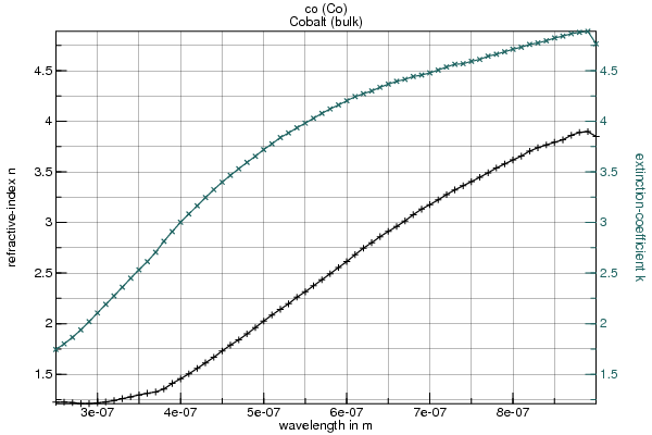
$ nk co .3.um .5.um 1.3.eV
co: 1.218+2.11i  300.nm (4.13.eV) (33333.3.cm^-1)
co: 2.025+3.72i  500.nm (2.48.eV) (20000.cm^-1)
co: 3.85+4.77i  (954.nm) 1.3.eV (10485.2.cm^-1)
$ nk Al 400.cm^-1
al: 75.77+1.7e+02i  (25.0.um) (0.0496.eV) 400.cm^-1
The ‘--plot’ option creates an encapsulated PostScript graph of n and k/n for the material specified.
nk --plot co
http://people.csail.mit.edu/jaffer/FreeSnell/co.png
Next: Program Interface, Previous: Material Databases, Up: FreeSnell [Contents][Index]
Designs are coded in Scheme language files. More than one design can
be specified in a design file, permitting sharing of code. A variety
of design examples are contained in the validation suites
dielectric.scm, metallic.scm, and granular.scm.
The graphs output by these suites are shown and discussed in
http://people.csail.mit.edu/jaffer/FreeSnell/dielectric.html,
http://people.csail.mit.edu/jaffer/FreeSnell/metallic.html, and
http://people.csail.mit.edu/jaffer/FreeSnell/granular.html
Next: Optical Stack, Previous: Specifying Designs, Up: Specifying Designs [Contents][Index]
The index-of-refraction of dielectric materials often varies little with wavelength. In these cases the index-of-refraction can be a number. It is often convenient to give a symbolic name to numbers. For example:
(define ZnS 2.2)
(define Ge 4.2)
After these definitions, layers can reference the identifiers:
(optical-stack
 (substrate 1)
 (layer      ZnS   528.64e-9)
 (layer      Ge    178.96e-9)
 (layer      ZnS   250.12e-9)
 (layer      Ge    123.17e-9)
             …
Sometimes the index-of-refraction is specified as a formula of wavelength. The Refractive index database at http://refractiveindex.info gives a formula for the refractive-index of the plastic PMMA over the range 0.4358.um to 1.052.um. We can use its formula as a Scheme function:
;; n^2 = C1 + C2*wl^2 + C3*wl^-2 + C4*wl^-4 + C5*wl^-6 + C6*wl^-8
(define PMMA
  (let ((C1 2.399964)
        (C2 -8.308636E-2)
        (C3 -1.919569E-1)
        (C4 8.720608E-2)
        (C5 -1.666411E-2)
        (C6 1.169519E-3))
    (lambda (w)                         ; wavelength in meters
      ;; wavelength in microns and limited to valid range
      (let* ((wl (max 0.4358 (min 1.052 (* w 1e6))))
             (wl^-2 (/ 1 wl wl)))
        (sqrt (+ C1
                 (* C2 wl wl)
                 (* (+ C3 (* (+ C4 (* (+ C5 (* C6
                                               wl^-2))
                                      wl^-2))
                             wl^-2))
                    wl^-2)))))))
For more compliated material properties FreeSnell retrieves the wavelength-dependent index-of-refraction by calling functions which interpolate values from the materials database (see Material Databases).
(require 'FreeSnell)
(require 'databases)
(require 'database-interpolate)

(define nk (open-database (or (getenv "NK_DATABASE_PATH") "nk.rwb")
            'rwb-isam))
(define ge (interpolate-from-table (open-table nk 'ge) 2))
(define zns (interpolate-from-table (open-table nk 'zns) 2))
…
In this example ge and zns can be passed as arguments to
layer and substrate.
For dielectric films embedded with spherical metal granules much smaller than the thickness of the film and the wavelengths under consideration, Maxwell Garnett Theory provides a means to calculate the effective n and k. The thickness of the granular film must be several times the granule size; otherwise the more complicated machinations of [Granfilm] are required.
The ir and ir0 arguments specify the indexes of refraction for the metallic and matrix materials respectively. Each can be either a (complex) number or function of one real argument returning a (complex) number. The real number q is the fractional volume occupied by the metal.
granular-IR returns a complex index-of-refraction (or
function returning a complex index-of-refraction) for the composite
layer.
If Au is a spectral function, the following three definitions are equivalent:
(define ruby-glass (granular-IR Au 8.0e-6 1.5))
(define (ruby-glass w) (granular-IR (Au w) 8.0e-6 1.5))
(define ruby-glass (lambda (w) (granular-IR (Au w) 8.0e-6 1.5)))
Next: Plot-response, Previous: Specifying Materials, Up: Specifying Designs [Contents][Index]
Returns a data structure combining its layer arguments. Each
layer is returned from a call to layer or substrate.
Substrate arguments must be first or last and default to having an
index-of-refraction of 1. A substrate has arbitrarily large
thickness, and is the source or sink of test inputs (radiation).
Returns a layer having the specified index-of-refraction and thickness.
If ir is a number, then the index-of-refraction is ir at
all wavelengths. If ir is a procedure then the
index-of-refraction at wavelength w is (ir
w).
If the number thick is smaller than 1/50, then it is taken as the actual thickness. Note that the effective optical thickness will be larger than the actual thickness because light is slowed by the index-of-refraction.
If the number thick is larger than 1/50, then the thickness is
thick times nominal divided by the real-part of the
index-of-refraction at nominal, where nominal is either
the third argument nom or the value set by the nominal
function. This is a convenient notation for the fractional optical
wavelengths often used to specify filter elements.
Layers specified by layer model the interference effects of
reflections of reflections. This is correct for thin layers or if the
modeled optical system will be illuminated by coherent light. But
layers thicker than several wavelengths have variations extremely
sensitive to incident angle.
Incoherent illumination will average over the wiggles. For these layers FreeSnell computes the transmitted and reflected power ratios, rather than E-fields.
Returns an incoherent layer having the specified index-of-refraction and thickness.
Returns a substrate having the specified index-of-refraction.
If ir is a number then the index-of-refraction is ir at
all wavelengths. If ir is a procedure then the
index-of-refraction at wavelength w is (ir
w).
If substrates are not specified, then their index-of-refraction defaults to 1 (vacuum).
To place a substrate between two sets of layers, use layer*
instead.
Sets the default nominal thickness to nom. Multiple
nominal commands are allowed interspersed with layer
commands. The arguments to optical-stack are considered in
order from the first to the last.
Inserts j copies of the sequence layer1, layer2, … into the stack.
Previous: Optical Stack, Up: Specifying Designs [Contents][Index]
One or more of arg1, arg2, … should be an optical
stack returned by optical-stack, or a value returned by a call
to IR. The other arguments should be values returned by the
functions in sections Ranges and Units, Traces, and
Other Outputs.
Plot-response creates a graph, data file, or color patches as
directed by its arguments. If more than one optical stack is given,
the same quantities are computed for each optical stack; but all are
plotted to a single graph.
Each color1, … should be a string naming a Resene color, a
saturate color, or a number between 0 and 100. If supplied, there
should be one color for each optical-stack. color1, …
default to black (0). If stack-colors is called more than
once, then its color arguments are appended together.
stack-colors causes the traces from each optical stack to be
drawn in its corresponding color.
Next: Traces, Previous: Plot-response, Up: Plot-response [Contents][Index]
Sets title for the run to str. If the string filebase is given, then it is used for the output filename root; otherwise str is used.
According to the symbol sym, sets the disposition of plots to be:
| eps | filebase.eps |
| ps | filebase.ps |
| png | filebase.png |
| jpg | filebase.jpg |
| jpeg | filebase.jpeg |
| filebase.pdf | |
| #t | views filebase.eps using ps:viewer. |
If output-format is not used, then the output-format defaults
to the value of top-level identifier *output-format*, which
defaults to #t.
If a pair of nonnegative exact integers, k1 and k2 follows sym, then the plot will be k1 pixels horizontally and k2 pixels vertically.
The output-format command does not affect the data written by
output-data.
If a string fnt is supplied, then it names the PostScript font
which will be used. The default value is Times.
If a nonnegative real number x follows the fnt, then x is the fontsize.
If two strings follow, then they are used as the templates whose printed representation using fnt is used to size the left and right margins respectively. If not specified, the templates default to ‘-.0123456789’.
If x is not specified and k1 is, then the font height will be k1/33. If neither is specified, then the font height will be 12.
The font command does not affect the data written by
output-data.
If the first character of file is ‘|’, then lines of data are piped to the stdin of the command line in file; otherwise a file of data is written to file.
str1 and str2 are printf format strings for the first number and the rest of the numbers printed on one line. If #f is passed, then the corresponding numbers are written with full Scheme precision and tab delimited.
Sets the ordinate range of the plot to low to high.
Sets the ordinate range of the plot to low to high decibels.
Sets the abscissa range of the plot to be linear from wavelengths 0.75*w to 1.25*w.
Sets the abscissa range of the plot to be linear from wavelengths w1 to w2.
Sets the abscissa range of the plot to be linear from wavelengths w1 to w2 in a graph rectangle from wavelengths g1 to g2.
Sets the abscissa range of the plot to be logarithmic from wavenumbers 0.666*w to 1.5*w.
Sets the abscissa range of the plot to be logarithmic from wavenumbers w1 to w2.
Sets the abscissa range of the plot to be linear from wavenumbers w1 to w2 in a graph rectangle from wavenumbers g1 to g2.
Sets the abscissa range of the plot to be linear from energy 0.666*x to 1.5*x electron Volts.
Sets the abscissa range of the plot to be linear from energy x1 to x2 electron Volts.
Sets the abscissa range of the plot to be linear from energy x1 to x2 electron Volts in a graph rectangle from energies g1 to g2 electron Volts.
Sets the abscissa range of the plot to be logarithmic from wavelengths 0.666*w to 1.5*w.
Sets the abscissa range of the plot to be logarithmic from wavelengths w1 to w2.
Sets the abscissa range of the plot to be logarithmic from wavelengths w1 to w2 in a graph rectangle from wavelengths g1 to g2.
Sets the abscissa range of the plot to be linear from angles 0.75*theta to 1.25*theta.
Sets the abscissa range of the plot to be linear from angles theta1 to theta2.
Places vertical arrows at abscissa coordinates w1, w2,
…. The marker command does not affect the data written
by output-data.
Sets the number of abscissa coordinates to k. The default value is 200.
Sets the number of abscissa coordinates to k. spacing is one of the (single-quoted) symbols ‘eV’, ‘ratio’, ‘wavelength’, or ‘wavenumber’, and determines the spacing of the samples. The default spacing is ‘ratio’ if the endpoint ratio is between 1.5 and 10000; and ‘wavelength’ otherwise.
Note that spacing does not need to match the abscissa scale. To generate 10 samples at evenly spaced wavelengths, do:
(samples 10 'wavelength)
Convolves the traces (before converting values to decibels) with a Gaussian filter having wavelength standard deviation sigma.
Next: Other Outputs, Previous: Ranges and Units, Up: Plot-response [Contents][Index]
These functions specify whether the plot holds angle constant and
varies wavelength; holds wavelength constant and varies angle; or
plots components of the index-of-refraction of a material. Multiple
invocations of any one of these functions puts all those specified
traces in one plot. To generate separate plots call
plot-response multiple times.
The type of a trace appearing in a plot is specified by a symbol. The first ten in this table are for separate polarizations. The rest average the two polarizations.
| T_s | S-plane transmission |
| R_s | S-plane reflection from top |
| B_s | S-plane reflection from bottom |
| A_s | S-plane absorption from top |
| L_s | S-plane absorption from bottom |
| T_p | P-plane transmission |
| R_p | P-plane reflection from top |
| B_p | P-plane reflection from bottom |
| A_p | P-plane absorption from top |
| L_p | P-plane absorption from bottom |
| T | tranmission |
| R | reflection from top |
| B | reflection from bottom |
| A | absorption from top |
| L | absorption from bottom |
A trace can also be a quoted scheme expression combining numbers and
the symbols listed above with the operators +, -,
*, /, ln, log_10, and average. The
following example computes the reflectivity relative to a substrate
reflectivity of 0.023:
(incident 45 '(/ (- R_p .023) .023))
A plot of trace1, trace2, … versus wavelength will be generated for radiation incident at angle degrees.
The angle argument can also be a list of angles in degrees. In this case the plots of trace1, trace2, … will be averaged over the angles given.
This is useful when profiling materials whose thicknesses are several times wavelengths of interest. Plots at a single angle of incidence can oscillate wildly with wavelength as the reflections go in and out of phase, constructively and destructively interfering.
A plot of trace1, trace2, … versus incident angle will be generated for radiation at wavelength w.
Plots characteristics of procedure substance versus wavelength. Symbols comp1, comp2, … determine the characteristics to be plotted:
n
k
k/n
Normal reflectance from a thick layer.
Previous: Traces, Up: Plot-response [Contents][Index]
Computes the color of trace at angle degrees from normal using CIE illuminant D65.
The following statement will cause plot-response to compute the
reflected color (average of both polarizations) at 30 degrees from the
surface normal.
(color-swatch 30 'R)
If there are any color-swatch statements passed to
plot-response, then a file named
filebase-color.png will be written containing 64x64
pixels color squares, one for each color computed. The squares are
arrayed horizontally in the order they are passed to
plot-response. Vertically, one such row is generated for each
optical stack.
The filebase string is that set by the title command.
For each stack, prints out the results of integrating each trace specified (token1, token2, …) at angle with "Key Centre for Photovoltaic Engineering UNSW - Air Mass 1.5 Global Spectrum" solar irradiance.
Next: About FreeSnell, Previous: Specifying Designs, Up: FreeSnell [Contents][Index]
(require 'fresnel-equations)
layers is a list of lists of index-of-refraction and thickness. The index-of-refraction may be a complex number or a procedure of wavelength (w) in meters returning a complex number.
Layers with negative thickness are modeled as incoherent (with positive thickness); otherwise as coherent (with inteference fringing).
The index-of-refraction of the top and bottom media are given by the first and last layers, which must have thickness 0. w is probe wavelength. th_i is the angle of the incident ray in radians.
Combine-layers returns a list of three non-negative real
numbers:
The transmitted and forward ratios sum to 1.0 if layers are all dielectric (lossless). The transmitted and reverse ratios sum to 1.0 if layers are all dielectric (lossless).
Negative w computes the S-polarization, else the P-polarization.
Complex numbers z1 and z2 are the indexes of refraction of the incident and opposite side of the boundary plane between two materials. th-i is the angle of incidence (from the normal of the boundary plane).
snell-law returns the exit angle (from normal) of an incident
ray impinging at th-i from normal.
If the ray undergoes total internal reflection, then the returned angle will not be real. If z1 and z2 are real, then the real part of the returned value will be pi/2 and represents a quickly decaying evanescent wave. Otherwise, the real part of the return value tends toward pi/2. I don’t know a physical interpretation of the imaginary part.
(snell-law 2.8 1.3 .1) ⇒ 216.71826868463917e-3
(snell-law 2.8 1.3 .3) ⇒ 689.9583515921762e-3
(snell-law 2.8 1.3 .4) ⇒ 994.9783891781343e-3
(snell-law 2.8 1.3 .5) ⇒ 1.5707963267948965-254.68865153727376e-3i
Next: Index, Previous: Program Interface, Up: FreeSnell [Contents][Index]
Free        Software
Fre snel    Equations
    Snell's Law
=========
FreeSnell
The author can be reached as ‘agj@alum.mit.edu’. The most recent information about FreeSnell can be found on the FreeSnell home page:
http://people.csail.mit.edu/jaffer/FreeSnell
Next: Using FreeSnell, Previous: About FreeSnell, Up: About FreeSnell [Contents][Index]
#! /bin/sh
wget http://groups.csail.mit.edu/mac/ftpdir/scm/slib-3c1-1.noarch.rpm
wget http://groups.csail.mit.edu/mac/ftpdir/scm/scm-5f4-1.x86_64.rpm
wget http://groups.csail.mit.edu/mac/ftpdir/scm/wb-2b4-1.x86_64.rpm
rpm -U slib-3c1-1.noarch.rpm scm-5f4-1.x86_64.rpm wb-2b4-1.x86_64.rpm
wget http://groups.csail.mit.edu/mac/ftpdir/scm/FreeSnell-1c4.zip
unzip FreeSnell-1c4.zip
(cd FreeSnell; ./configure --prefix=/usr/local/; make install)
#! /bin/sh
wget http://groups.csail.mit.edu/mac/ftpdir/users/jaffer/slib.zip
wget http://groups.csail.mit.edu/mac/ftpdir/users/jaffer/scm.zip
wget http://groups.csail.mit.edu/mac/ftpdir/users/jaffer/wb.zip
wget http://groups.csail.mit.edu/mac/ftpdir/scm/FreeSnell.zip
unzip slib.zip
unzip scm.zip
unzip wb.zip
unzip FreeSnell.zip
(cd slib; ./configure --prefix=/usr/local/; make install)
(cd scm; ./configure --prefix=/usr/local/;
 make scmlit; make scm5; make mydlls; make wbscm.so; make install)
(cd FreeSnell; ./configure --prefix=/usr/local/; make install)
Previous: Installation, Up: About FreeSnell [Contents][Index]
To run FreeSnell from the C:\Program Files\SCM\FreeSnell diretory, click on the FreeSnell desktop icon. In Unix, from the ‘FreeSnell’ directory run ‘scm’.
You can then type expressions to the SCM interpreter. To run FreeSnell’s regression suites type:
(load "dielectric.scm")
(dielectric)
(load "metallic.scm")
(metallic)
(load "granular.scm")
(granular)
(load "coherence.scm")
(coherence)
(load "polyethylene.scm")
(polyethylene)
I set up design directories as peers of ‘FreeSnell’; that is, both are subdirectories of the same directory. I find it useful to put related designs in one directory.
In order to load FreeSnell files, you should create a local SLIB catalog (named usercat) within the design directory or your HOME directory. This catalog translates symbols to the pathnames of FreeSnell files. Here is the usercat included in the FreeSnell distribution, which is suitable to copy to design directories which are peers of FreeSnell:
;;; "usercat": SLIB catalog additions for thin-film optics. -*-scheme-*-
(
 (fresnel-equations     . "fresneleq")
 (optic-compute         . "opticompute")
 (optic-plot            . "optiplot")
 (optic-color           . "opticolr")
 (video-processing	. "video")
 (optic-solar		. "solar-am15")
 (FreeSnell aggregate optic-compute optic-plot optic-color optic-solar)
 )
Design files can then load FreeSnell with the expression:
(require 'FreeSnell)
Realize that this usercat file assumes that the FreeSnell directory is named FreeSnell. If your FreeSnell directory is named something else, then substitute its name for FreeSnell in the right hand side of lines in usercat.
Previous: About FreeSnell, Up: FreeSnell [Contents][Index]
| Jump to: | A C D E F G H I L M N O P R S T W |
|---|
| Jump to: | A C D E F G H I L M N O P R S T W |
|---|