While Markov Decision Processes (MDPs) are quite general and expressive models for reasoning about actions in the face of uncertainty, they don't scale well to the very large state spaces in which we're really interested. In particular, while exact reasoning algorithms for MDPs run in time polynomial in the size of the total state space, many problems of interest to AI researchers are best written in terms of discrete state variables. The total state space, then, is the cross product of the individual variables and reasoning methods are then exponential in the number of state variables. For example, we are currently working with a model of a package delivery problem that has a total state space of roughly 2500 states.
A number of decomposition, abstraction, and approximation techniques to address this exponential complexity have been proposed by various researchers. (A brief and far from complete bibliography of related papers on the subject can be found here.) Our current belief is that a true solution to this problem will involve parts of many of these proposals (or, ideally, an as yet unconceived generalization that encompasses all of these ideas). We are particularly interested in examining ideas based on
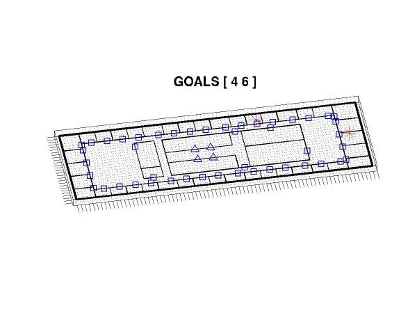
Consider the following maze world, roughly modeled after the seventh floor of the Artificial Intelligence lab building at MIT (this is actually a small subset of the package delivery problem). The blue squares indicate the locations of doors and the blue triangles indicate the elevators; black lines are impermeable walls. Under a simplistic model of robot navigation, the agent can move in any of the cardinal directions with high probability of success (0.9 in this world dynamic), except where blocked by walls or locked doors. When the robot fails to move in the desired direction, it finds itself in another (accessible) adjacent cell with uniform probability.
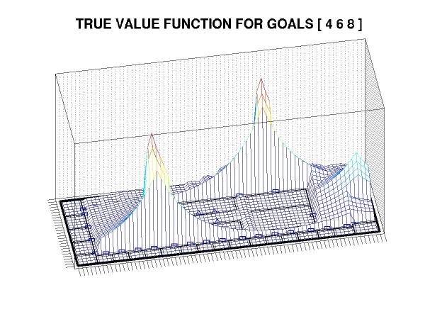
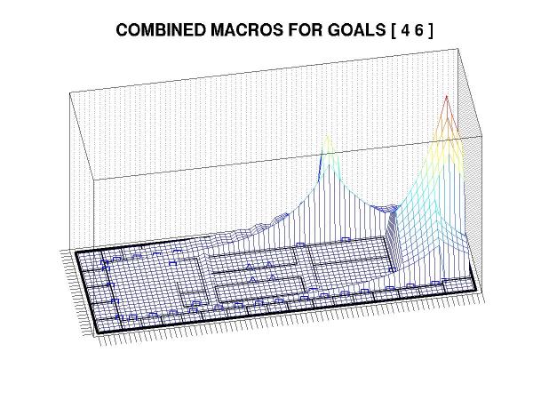
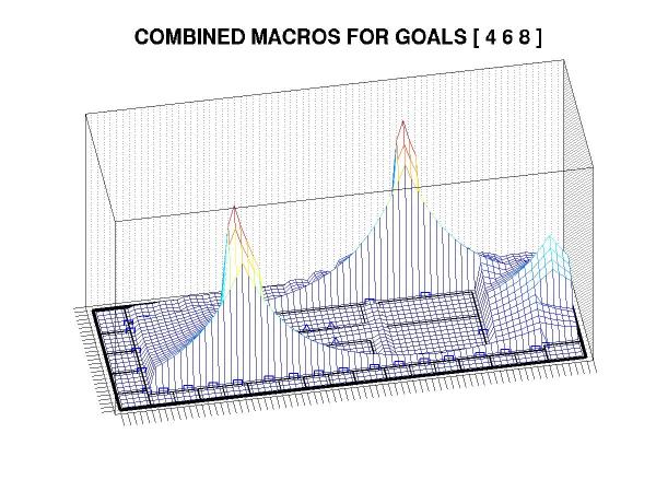
Suppose that we wish the robot to deliver packages to the two locations denoted with red asterisks in the map. In an MDP framework, we associate a reward with each goal state and plan a course of action so as to maximize the expected total reward. Notably, in standard techniques all reward sources are integrated simultaneously and the resulting plan depends on the precise relationships of reward magnitudes between the different goals. We are, instead, interested in approaches to decomposing the reward function into components associated with individual sub-goals. For example, a goal-specific plan (also known as a macro action or, more generally, an option) for reaching goal state 4 would look like:
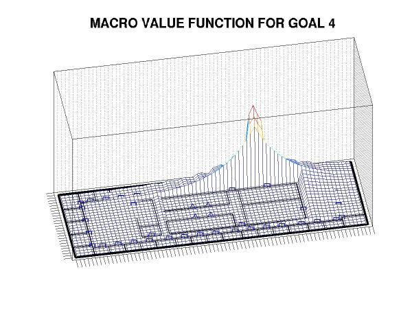
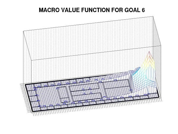
Technically, this structure is a value function, which represents the expected discounted reward achievable from each state by following the policy; in essence, the agent follows the gradient of this function to seek a goal state. For more details on the relationships of plans to value functions, see Puterman's text.
Similarly, a plan for achieving the sub-goal associated with state 6 looks like:
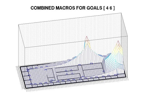
Furthermore, we can easily change the relative weights of the goal states in response to changing environmental demands. This plot would again require a full recomputation of the MDP but we produce it cheaply, using only the cached macros for the individual goal states:
Of course, it really would be too much to hope that we could get all of that for free. The nearly inevitable catch is that this approach can produce sub-optimal plans -- sometimes substantially so. The fundamental problem is that the goal states interact in complex ways and, in general, the problem of trading off between different goals can be NP-hard (more specifically, if you have to achieve a number of different goal states in succession and need to decide what order to take them in, then you're effectively dealing with the TSP). Such decisions cannot (to the best of anyone's knowledge) be resolved purely with local information, so it's some consolation to realize that suboptimality is inevitable given the runtime constraints that we've applied.
There is, however, still the question of just how suboptimal a plan our heuristic produces. It is not yet clear whether we can bound this quantity, though we have evidence to indicate that the loss is generally small. For example, here is the exact plan corresponding to the last example, above: