IEEE Transactions on Pattern Analysis and Machine Intelligence, Vol. 33, No. 12, December 2011
Nonparametric Scene Parsing via Label Transfer
Ce Liu1 Jenny Yuen2 Antonio Torralba2
1Microsoft Research New England 2Massachusetts Institute of Techonolgy
Download the code and database
Abstract |
| While there has been a lot of recent work on object recognition and image understanding, the focus has been on carefully establishing mathematical models for images, scenes, and objects. In this paper, we propose a novel, nonparametric approach for object recognition and scene parsing using a new technology we name label transfer. For an input image, our system first retrieves its nearest neighbors from a large database containing fully annotated images. Then, the system establishes dense correspondences between the input image and each of the nearest neighbors using the dense SIFT flow algorithm, which aligns two images based on local image structures. Finally, based on the dense scene correspondences obtained from SIFT flow, our system warps the existing annotations and integrates multiple cues in a Markov random field framework to segment and recognize the query image. Promising experimental results have been achieved by our nonparametric scene parsing system on challenging databases. Compared to existing object recognition approaches that require training classifiers or appearance models for each object category, our system is easy to implement, has few parameters, and embeds contextual information naturally in the retrieval/alignment procedure |
Scene parsing, or recognizing and segmenting objects in an image, is one of the core problems of computer vision. Traditional approaches to object recognition begin by specifying an object model, such as template matching, constellations, bags of features, or shape models, etc. These approaches typically work with a fixed number of object categories and require training generative or discriminative models for each category from training data. In the parsing stage, these systems try to align the learned models to the input image and associate object category labels with pixels, windows, edges, or other image representations. Recently, context information has also been carefully modeled to capture the relationship between objects at the semantic level. Encouraging progress has been made by these models on a variety of object recognition and scene parsing tasks.
Introduction

|
| Fig 1. For a query image (a), our system finds the top matches (b) (three are shown here) using scene retrieval and a SIFT flow matching algorithm. The annotations of the top matches (c) are transferred and integrated to parse the input image, as shown in (d). For comparison, the ground-truth user annotation of (a) is shown in (e). |
However, these learning-based methods do not, in general, scale well with the number of object categories. For example, to include more object categories in an existing system, we need to train new models for the new categories and, typically, adjust system parameters. Training can be a tedious job if we want to include thousands of object categories in a scene parsing system. In addition, the complexity of contextual relationships among objects also increases rapidly as the quantity of object categories expands.
Recently, the emergence of large databases of images has opened the door to a new family of methods in computer vision. Large database-driven approaches have shown the potential for nonparametric methods in several applications. Instead of training sophisticated parametric models, these methods try to reduce the inference problem for an unknown image to that of matching to an existing set of annotated images.
In this paper, we propose a novel, nonparametric scene parsing system to transfer the labels from existing samples in a large database to annotate an image, as illustrated in Fig. 1. For a query image (Fig. 1a), our system first retrieves the top matches in a large, annotated image database using a combination of GIST matching [Oliva 2001] and SIFT flow [Liu 2011]. Since these top matches are labeled, we transfer the annotation (Fig. 1c) of the top matches to the query image and obtain the scene parsing result in (Fig. 1d). For comparison, the groundtruth user annotation of the query is displayed in (Fig. 1e). Our system is able to generate promising scene parsing results if images from the same scene type as the query are retrieved in the annotated database.
However, it is nontrivial to build an efficient and reliable scene parsing system using dense scene alignment. To account for the multiple annotation suggestions from the top matches, a Markov random field model is used to merge multiple cues (e.g., likelihood, prior, and spatial smoothness) into a robust annotation. Promising experimental results are achieved on images from the LabelMe database [Russell 2008].
Our goal is to explore the performance of scene parsing through the transfer of labels from existing annotated images, rather than building a comprehensive object recognition system. We show, however, that the performance of our system outperforms existing approaches [Dalas 2005, Shotton 2011] on our databases.
System Overview
The core idea of our nonparametric scene parsing system is recognition-by-matching. To parse an input image, we match the visual objects in the input image to the images in a database. If images in the database are annotated with object category labels and if the matching is semantically meaningful, i.e., building corresponds to building, window to window, person to person, then we can simply transfer the labels of the images in the database to parse the input. Nevertheless, we need to deal with many practical issues in order to build a reliable system.
Fig. 2 shows the pipeline of our system, which consists of the following three algorithmic modules:
- Scen reetrieval: Given a query image, use scene retrieval techniques to find a set of nearest neighbors that share similar scene configuration (including objects and their relationships) with the query.
- Dense scene alignment: Establish dense scene correspondence between the query image and each of the retrieved nearest neighbors. Choose the nearest neighbors with the top matching scores as voting candidates.
- Label transfer: Warp the annotations from the voting candidates to the query image according to estimated dense correspondence. Reconcile multiple labeling and impose spatial smoothness under a Markov random field (MRF) model.

|
| Figure 2. System pipeline.There are three key algorithmic components (rectangles) in our system: scene retrieval, dense scene alignment, and label transfer. The ovals denote data representations. |
Although we are going to choose concrete algorithms for each module in this paper, any algorithm that fits to the module can be plugged into our nonparametric scene parsing system. For example, we use SIFT flow for dense scene alignment, but it would also suffice to use sparse feature matching and then propagate sparse correspondences to produce dense counterparts.
A key component of our system is a large, dense, and annotated image database.1 In this paper, we use two sets of databases, both annotated using the LabelMe online annotation tool [Russell 2008], to build and evaluate our system. The first is the LabelMe Outdoor (LMO) database [Liu 2009], containing 2,688 fully annotated images, most of which are outdoor scenes including street, beach, mountains, fields, and buildings. The second is the SUN database [Xiao 2010], containing 9,566 fully annotated images, covering both indoor and outdoor scenes; in fact, LMO is a subset of SUN. We use the LMO database to explore our system in-depth, and also report the results on the SUN database.

|
| Figure 3. Top: The per-pixel frequency counts of the object categories in our data set (sorted in descending order). The color of each bar is the average RGB value of each object category from the training data with saturation and brightness boosted for visualization. Bottom: The spatial priors of the object categories in the database. White means zero and the saturated color means high probability. |
Before jumping into the details of our system, it is helpful to look at the statistics of the LMO database. The 2,688 images in LMO are randomly split into 2,488 for training and 200 for testing. We chose the top 33 object categories with the most labeled pixels. The pixels that are not labeled, or labeled as other object categories, are treated as the 34th category: “unlabeled.” The per pixel frequency count of these object categories in the training set is shown at the top of Fig. 3. The color of each bar is the average RGB value of the corresponding object category from the training data with saturation and brightness boosted for visualization purposes. The top 10 object categories are sky, building, mountain, tree, unlabeled, road, sea, field, grass, and river. The spatial priors of these object categories are displayed at the bottom of Fig. 3, where white denotes zero probability and the saturation of color is directly proportional to its probability. Note that, consistent with common knowledge, sky occupies the upper part of the image grid and field occupies the lower part. Furthermore, there are only limited samples for the sun, cow, bird, and moon classes.
Scene Retrieval
The objective of scene retrieval is to retrieve a set of nearest neighbors in the database for a given query image. There exist several ways for defining a nearest neighbor set. The most common definition consists of taking the K closest points to the query (K-NN). Another model, ε-NN, widely used in texture synthesis [Efros 1999, Liang 2001], considers all of the neighbors within (1+ε) times the minimum distance from the query. We generalize these two types to <K,ε>-NN, and define it as

As ε→∞, <K,ε>-NN is reduced to K-NN. As K→∞, <K,ε>-NN is reduced to ε-NN. However, <K,ε>-NN representation gives us the flexibility to deal with the density variation of the graph, as shown in Fig. 4. We will show how K affects the performance in the experimental section. In practice, we found that ε=5 is a good parameter and we will use it through our experiments. Nevertheless, dramatic improvement of <K,ε>-NN over K-NN is not expected as sparse samples are few in our databases.
 |
| Fig. 4. An image database can be nonuniform as illustrated by some random 2D points. The green node (A) is surrounded densely by neighbors, whereas the red node (B) resides in a sparse area. If we use K-NN (K=5), then some samples (orange nodes) far away from the query (B) can be chosen as neighbors. If, instead, we use ε-NN and choose the radius as shown in the picture, then there can be too many neighbors for a sample such as (A). The combination, <K,ε>-NN, shown as gray-edges, provides a good balance for these two criteria. |
We have not yet defined the distance function dist(·,·) between two images. Measuring image similarities/distances is still an active research area; a systematic study of image features for scene recognition can be found in [Xiao 2010]. In this paper, three distances are used: euclidean distance of GIST [Oliva 2001], spatial pyramid histogram intersection of HOG visual words [Lazebnik 2006], and spatial pyramid histogram intersection of the ground-truth annotation. For the HOG distance, we use the standard pipeline of computing HOG features on a dense grid and quantizing features to visual words over a set of images using k-means clustering. The ground truthbased distance metric is used to estimate an upper bound of our system for evaluation purposes. Both the HOG and the ground truth distances are computed in the same manner. The ground truth distance is computed by building histograms of pixel-wise labels. To include spatial information, the histograms are computed by dividing an image into 2×2 windows and concatenating the four histograms into a single vector. Histogram intersection is used to compute the ground truth distance. We obtain the HOG distance by replacing pixel-wise labels with HOG visual words.
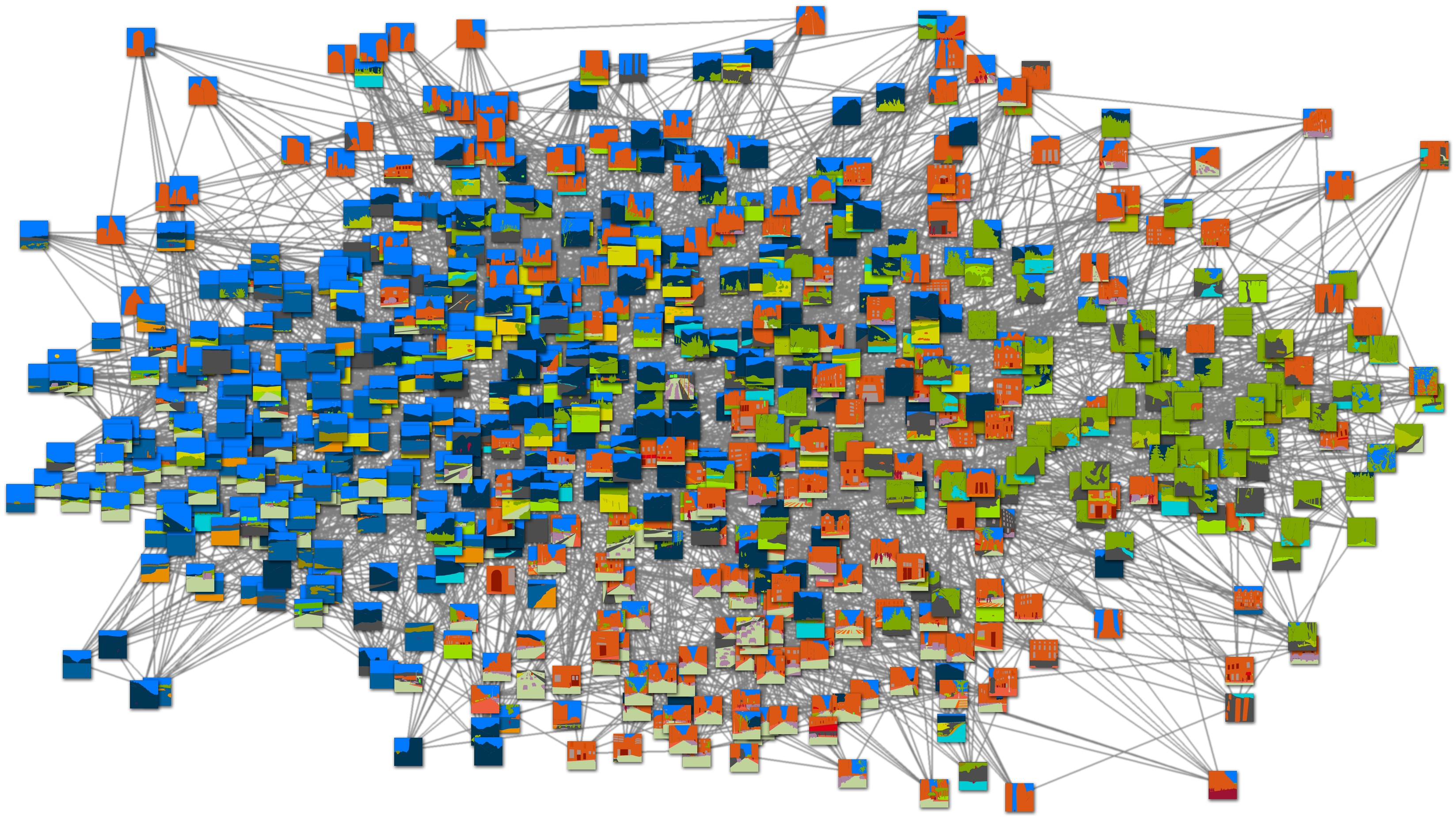
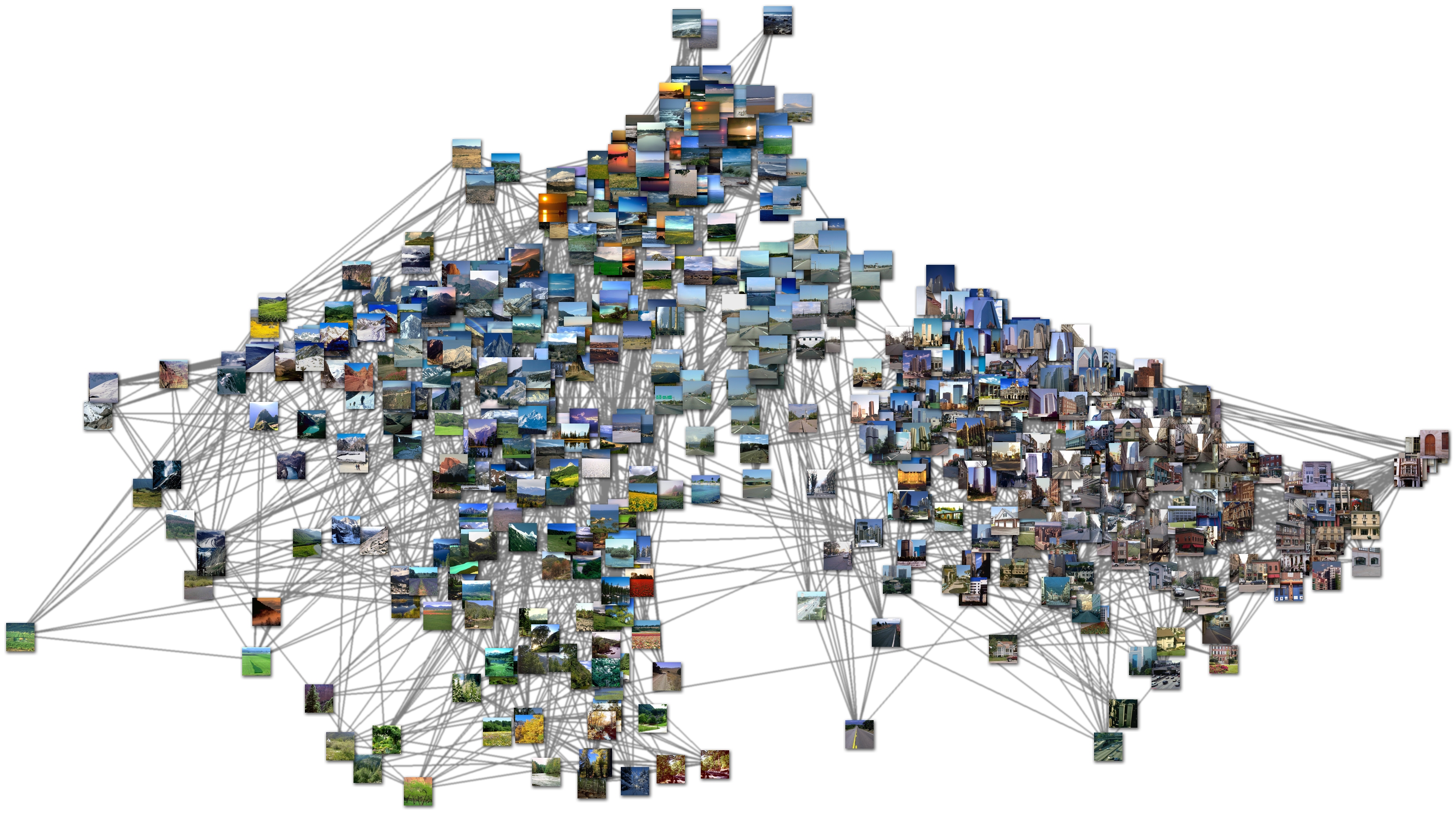
In Fig. 5, we show the importance of the distance metric as it defines the neighborhood structure of the large image database. We randomly selected 200 images from the LMO database and computed pair-wise image distances using GIST (top) and the ground-truth annotation (bottom). Then, we use multidimensional scaling (MDS) [Borg 2005] to map these images to points on a 2D grid for visualization. Although the GIST descriptor is able to form a reasonably meaningful image space where semantically similar images are clustered, the image space defined by the ground-truth annotation truly reveals the underlying structures of the image database. This will be further examined in the experimental section.

|
|
| (a) Graph structure revealed by GIST distance (click to view the full-size) | (b) The same as (a), showing ground-truth annotation (click to view the full-size) |
|

|
| (c) The same as (d), showing RGB images (click to view the full-size) | (d) Graph structure revealed by the distance on ground-truth annotation (click to view the full-size) |
| Fig. 5. The structure of a database depends on image distance metric. Top: The <K,ε>-NN graph of the LabelMe Outdoor database visualized by scaled MDS using GIST feature as distance. Bottom: The <K,ε>-NN graph of the same database visualized using the pyramid histogram intersection of ground-truth annotation as distance. Left: RGB images; right: annotation images. Notice how the ground-truth annotation emphasizes the underlying structure of the database. In (c) and (d), we see that the image content changes from urban, streets (right), to highways (middle), and to nature scenes (left) as we pan from right to left. Eight hundred images are randomly selected from LMO for this visualization | |
SIFT flow algorithm
As our goal is to transfer the labels of existing samples to parse an input image, it is essential to find the dense correspondence for images across scenes. In our previous work [Liu 2008], we have demonstrated that SIFT flow is capable of establishing semantically meaningful correspondences among two images by matching local SIFT descriptors. We further extended SIFT flow into a hierarchical computational framework to improve the performance [Liu 2009]. In this section, we will provide a brief explanation of the algorithm; for a detailed description, we refer to [Liu 2011] and this link.
We formulate SIFT flow the same as optical flow with the exception of matching SIFT descriptors instead of RGB values. Therefore, the objective function of SIFT flow is very similar to that of optical flow. Let p=(x,y) be the grid coordinate of images, and w(p)=(u(p),v(p)) be the flow vector at p. We only allow u(p) and v(p) to be integers and we assume that there are L possible states for u(p) and v(p), respectively. Let s1 and s2 be two SIFT images that we want to match. Set ε contains all the spatial neighborhoods (a four-neighbor system is used). The energy function for SIFT flow is defined as:

which contains a data term, small displacement term and smoothness term (a.k.a. spatial regularization). The data term on line 1 constrains the SIFT descriptors to be matched along with the flow vector w(p). The small displacement term on line 2 constrains the flow vectors to be as small as possible when no other information is available. The smoothness term on line 3 constrains the flow vectors of adjacent pixels to be similar. In this objective function, truncated L1 norms are used in both the data term and the smoothness term to account for matching outliers and flow discontinuities, with t and d as the threshold, respectively.
While SIFT flow has demonstrated the potential for aligning images across scenes [Liu 2008], the original implementation scales poorly with respect to image sizes. In SIFT flow, a pixel in one image can literally match to any pixels in the other image. Suppose the image has h2 pixels, then L ≈ h, and the time and space complexity of this dual-layer BP is O(h4). For example, the computation time for 145×105 images with an 80×80 search window is 50 seconds. It would require more than two hours to process a pair of 256×256 images with a memory usage of 16GB to store the data term. To address the performance drawback, a coarse-to-fine SIFT flow matching scheme was designed to significantly improve the performance. As illustrated in Fig. 6, the basic idea consists of estimating the flow at a coarse level of image grid, and then gradually propagating and refining the flow from coarse to fine; please refer to [Liu 2011] for details. As a result, the complexity of this coarse-to-fine algorithm is O(h2 log h), a significant speed up compared to O(h4). Moreover, we double η and retain α and d as the algorithm moves to a higher level of pyramid in the energy minimization. Using the proposed coarse-to-fine matching scheme and modified distance transform function, the matching between two 256×256 images takes 31 seconds on a workstation with two quad-core 2.67 GHz Intel Xeon CPUs and 32 GB memory, in a C++ implementation.
 |
Fig 6. An
illustration of coarse-to-fine SIFT flow matching on pyramid.
The green square is the searching window for pk at each pyramid
level k. For simplicity only one image is shown here,
where pk is on image s1, and ck and w(pk) are on image
s2. |
Label transfer
Now that we have a large database of annotated images and a technique for establishing dense correspondences across scenes, we can transfer the existing annotations to parse a query image through dense scene alignment. For a given query image, we retrieve a set of <K,ε>-nearest neighbors in our database using GIST matching [Oliva 2011]. We then compute the SIFT flow from the query to each nearest neighbor, and use the achieved minimum energy to rerank the <K,ε>-nearest neighbors. We further select the top M reranked retrievals (M ≤ K) to create our voting candidate set. This voting set will be used to transfer its contained annotations into the query image. This procedure is illustrated in Fig. 7.
 |
| Fig. 7. For a query image, we first find a <K,ε>-nearest neighbor set in the database using GIST matching [34]. The nearest neighbors are reranked using SIFT flow matching scores, and form a top M-voting candidate set. The annotations are transferred from the voting candidates to parse the query image |
Under this setup, scene parsing can be formulated as the following label transfer problem: for a query image I with its corresponding SIFT image s, we have a set of voting candidates {si, ci, wi}i=1:M, where si, ci, and wi are the SIFT image, annotation, and SIFT flow field (from s to si) of the ith voting candidate, respectively. ci is an integer image where ci(p)∈{1,...,L} is the index of object category for pixel p. We want to obtain the annotation c for the query image by transferring ci to the query image according to the dense correspondence wi.
We build a probabilistic Markov random field model to integrate multiple labels, prior information of object category, and spatial smoothness of the annotation to parse image I. Similarly to that of [Shotton 2011], the posterior probability is defined as:
![]()
where Z is the normalization constant of the probability. This posterior contains three components, i.e., likelihood, prior, and spatial smoothness.
The likelihood term is defined as

where Ωp,l={i;ci(p+w(p))=l}, l=1,...,L, is the index set of the voting candidates whose label is l after being warped to pixel p. τ is set to be the value of the maximum difference of SIFT feature: τ = maxs1,s2,p||s1(p)-s2(p)||.
The prior term λ(c(p)=l) indicates the prior probability that object category l appears at pixel p. This is obtained from counting the occurrence of each object category at each location in the training set:

where histl(p) is the spatial histogram of object category l.
The smoothness term is defined to bias the neighboring pixels into having the same label in the event that no other information is available, and the probability depends on the edge of the image: The stronger luminance edge, the more likely it is that the neighboring pixels may have different labels:

where ϒ=(2<||I(p)-I(q)||2>)-1 [Shotton 2011].
Notice that the energy function is controlled by four parameters, K and M that decide the mode of the model and α and β that control the influence of spatial prior and smoothness. Once the parameters are fixed, we again use the BP-S algorithm to minimize the energy. The algorithm converges in two seconds on a workstation with two quadcore 2.67 GHz Intel Xeon CPUs.
A significant difference between our model and that in [43] is that we have fewer parameters because of the nonparametric nature of our approach, whereas classifiers were trained in [Shotton 2011]. In addition, color information is not included in our model at the present as the color distribution for each object category is diverse in our databases.
Results on LMO
Extensive experiments were conducted to evaluate our system. We shall first report the results on a small scale database which we will refer to as the LabelMe Outdoor (LMD) database in Section 5.1; this database will aid us for an in-depth exploration of our model. Furthermore, we will report results on the SUN database, a larger and more challenging data set in Section 5.2.
|
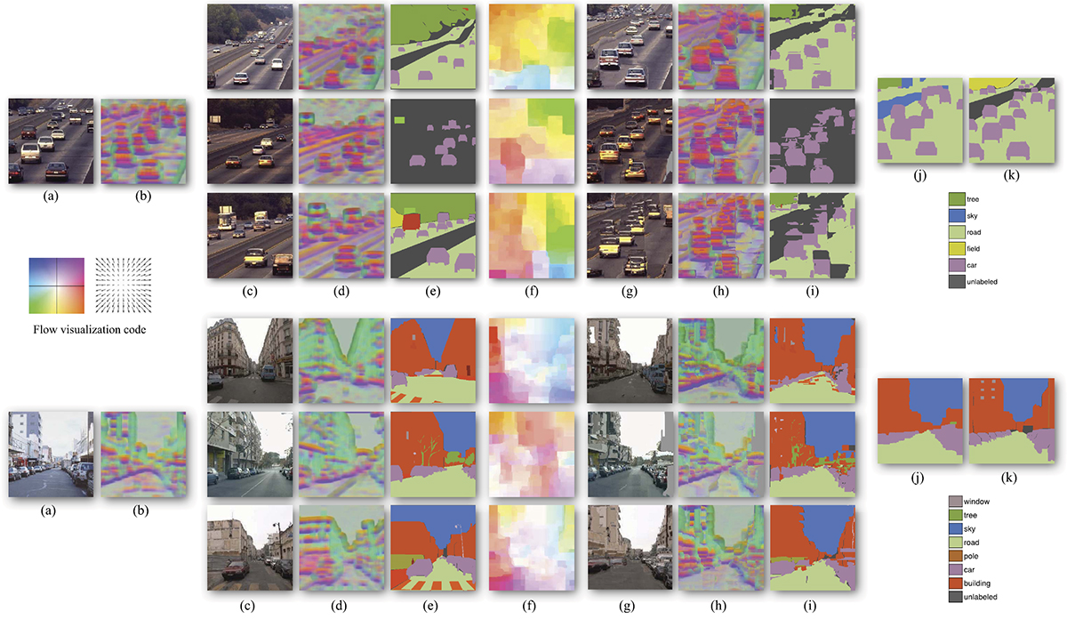
| Fig 8. System overview. For a query image, our system uses scene retrieval techniques such as [Shotton 2011] to find <K,ε>-nearest neighbors in our database. We apply coarse-to-fine SIFT flow to align the query image to the nearest neighbors, and obtain top M as voting candidates (M = 3 here). (c), (d), (e): The RGB image, SIFT image and user annotation of the voting candidates. (f): The inferred SIFT flow field, visualized using the color scheme shown on the left (hue: orientation; saturation: magnitude). (g), (h), and (i) are the warped version of (c), (d), (e) with respect to the SIFT flow in (f). Notice the similarity between (a) and (g), (b) and (h). Our system combines the voting from multiple candidates and generates scene parsing in (j) by optimizing the posterior. (k): The ground-truth annotation of (a). |

|
| Fig. 9. The ROC curve of each individual pixel-wise binary classifier (Click to zoom in). Red curve: Our system after being converted to binary classifiers; blue curve: the system in [8]. We used the convex hull to make the ROC curves strictly concave. The number (n,m) underneath the name of each plot is the quantity of the object instances in the test and training set, respectively. For example, (170, 2,124) under “sky” means that there are 170 test images containing sky, and 2,124 training images containing sky (there are in total 2,488 training images and 200 test images). Our system obtains reasonable performance for objects with sufficient samples in both training and test sets, e.g., sky, building, mountain, and tree. We observe truncation in the ROC curves where there are not enough test samples, e.g., field, sea, river, grass, plant, car, and sand. The performance is poor for objects without enough training samples, e.g., crosswalk, sign, boat, pole, sun, and bird. The ROC does not exist for objects without any test samples, e.g., desert, cow, and moon. In comparison, our system outperforms or equals [Dalal 2006] for all object categories except for grass, plant, boat, person, and bus. The performance of [Dalal 2006] on our database is low because the objects have drastically different poses and appearances. |

|
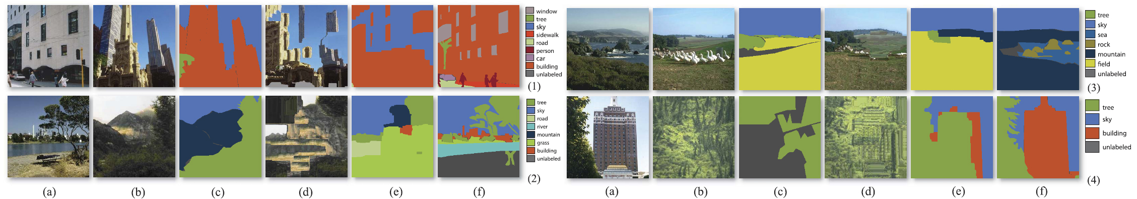
| Fig. 10. Some scene parsing results output from our system (Click to zoom in). (a): Query image, (b): the best match from nearest neighbors, (c): the annotation of the best match, (d): the warped version of (b) according to the SIFT flow field, (e): the inferred per-pixel parsing after combining multiple voting candidates, (f): the ground truth annotation of (a). The dark gray pixels in (f) are “unlabeled.” Notice how our system generates a reasonable parsing even for these “unlabeled” pixels. |
|
| Fig. 11. Some typical failures (Click to zoom in). Our system fails when no good matches can be retrieved in the database. In (2), for example, since the best matches do not contain river, the input image is mistakenly parsed as a scene of grass, tree, and mountain in (e). The ground-truth annotation is in (f). The failure may also come from ambiguous annotations, for instance in (3), where the system outputs field for the bottom part, whereas the ground-truth annotation is mountain. |

|
| Fig. 12. We study the performance of our system in depth (Click to zoom in). (a) Our system with the parameters optimized for pixel-wise recognition rate. (b) Our system, matching RGB instead of matching dense SIFT descriptors. (c) The performance of [Shotton 2011] with the Markov random field component turned off, trained and tested on the same data sets as (a). In (d), (e), (f), we show the importance of SIFT flow matching and the MRF for label transfer by turning them on and off. In (g) and (h), we show the system performance affected by other scene retrieval methods. The performance in (h) shows the upper limit of our system, by adopting ideal scene retrieval using ground-truth annotation (of course, the ground-truth annotation is not available in practice). |
|
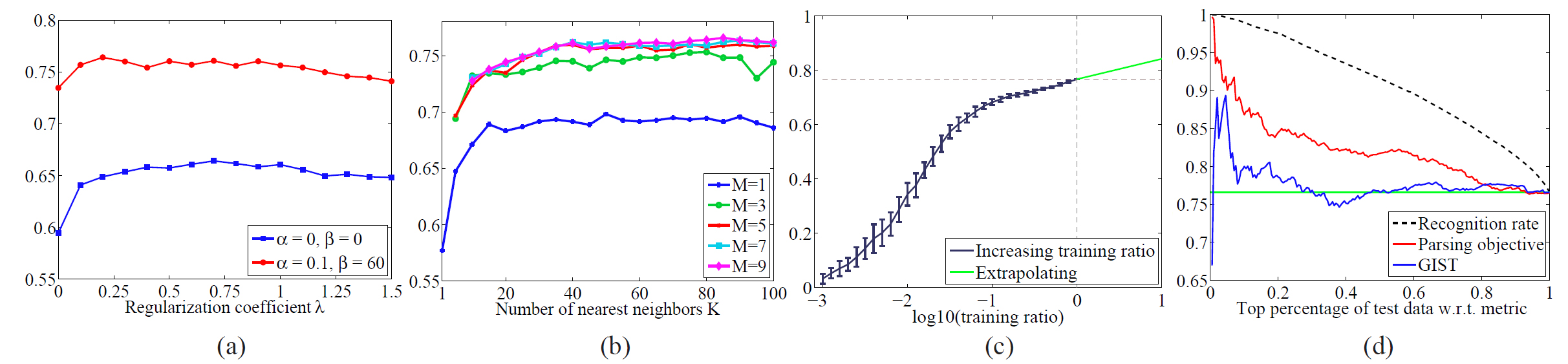
| Fig. 13 (Click to zoom in). (a): Recognition rate as a function of the spatial smoothness coefficient λ under two settings for α and β. (b): Recognition rate as a function of number of nearest neighbors K and the number of voting candidates M. Clearly, prior and spatial smoothness help improve the recognition rate. The fact that the curve drops down as we further increase K indicates that SIFT flow matching cannot replace scene retrieval. (c): Recognition rate as a function of the log training ratio while the test set is fixed. A subset of training samples are randomly drawn from the entire training set according to the training ratio to test how the performance depends on the size of the database. (d): Recognition rate as a function of the proportion of the top ranked test images according to metrics including GIST, the parsing objective in (5), and the recognition rate (with ground-truth annotation). The black, dashed curve with recognition rate as sorting metric is the ideal case, and the parsing objective is better than GIST. These curves suggests the system is somewhat capable of distinguishing good parsing results from bad ones. |
Results on SUN
We further evaluated the performance of our system on the SUN database [Xiao 2010], which contains 9,556 images of both indoor and outdoor scenes. This database contains a total of 515 object categories; the pixel frequency counts for the top 100 categories are displayed in Fig. 15a. The data corpus is randomly split into 8,556 images for training and 1,000 for testing. The structure of the database is visualized in Fig. 14 using the same technique to plot Fig. 5, where the image distance is measured by the ground-truth annotation. Notice the clear separation of indoor (left) and outdoor (right) scenes in this database. Moreover, the images are not evenly distributed in the space; they tend to reside around a few clusters. This phenomenon is consistent with human perception, drawing a clear separation between outdoor and indoor images.
| (a) Nodes and edges |

|
| (b) RGB images |

|
| (c) Ground-trth annotation |

|
| Fig. 14. Visualization of the SUN database [Xiao 2011] using 1,200 random images (Click to zoom in). Notice that the SUN database is larger but not necessarily denser than the LMO database. We use the spatial pyramid histogram intersection distance of the ground-truth annotation to measure the distance between the images and project them to a 2D space using scaled multidimensional scaling. Clearly, the images are clustered to indoor (left) and outdoor (right) scenes, and there is smooth transition in between. In the outdoor cluster, we observe the change from garden, street, to mountain and valley as we move from top to bottom. Please visit http://people.csail.mit.edu/celiu/LabelTransfer/ to see the full resolution of the graphs. | |

|
| Fig. 15. The per-class recognition rate of running our system on the SUN database (Click to zoom in). (a) Pixel-wise frequency histogram of the top 100 object categories. (b): The per-class recognition rate when the ground-truth annotation is used for scene retrieval. This is the upper limit performance that can be achieved by our system. (c) and (d): Per-class recognition rate using HOG and GIST for scene retrieval, respectively. The HOG visual words features generate better results for this larger database. |
Some scene parsing results are displayed in Fig. 16 in the same format as Fig. 10. Since the SUN database is a superset of the LabelMe Outdoor database, the selection of results is slightly biased toward indoor and activity scenes. Overall, our system performs reasonably well in parsing these challenging images.
We also plot the per-class performance in Fig. 15. In Fig. 15a, we show the pixel-wise frequency count of the top 100 object categories. Similarly toLMO,this prior distribution is heavily biased toward stuff-like classes, e.g., wall, sky, building, floor, and tree. In Fig. 15b, the performance is achieved when the ground-truth annotation is used for scene retrieval. Again, the average 64.45 percent recognition rate reveals the upper limit and the potential of our system in the idealized case of perfect nearest neighbor retrieval. In Figs. 15c and 15d, the performance using HOG and GIST features for scene retrieval is plotted, suggesting that the HOG visual words features outperform GIST for this larger database. This is consistent with the discovery that the HOG feature is the best among a set of features, including GIST, in scene recognition in the SUN database [Xiao 2010].

|
| Fig. 16. Some scene parsing results on the SUN database (Click to zoom in; following the same notation as in Fig. 10). Note that the LabelMe Outdoor database is a subset of the SUN database, but the latter contains a larger proportion of indoor and activity-based scenes. As it is in all cases, the success of the final parsing depends on the semantic similarity of the query in (a) to the warped support image (d). Examples (10) and (11) are two failure examples where many people are not correctly labeled. |
Conclusion
We have presented a novel, nonparametric scene parsing system to integrate and transfer the annotations from a large database to an input image via dense scene alignment. A coarse-to-fine SIFT flow matching scheme is proposed to reliably and efficiently establish dense correspondences between images across scenes. Using the dense scene correspondences, we warp the pixel labels of the existing samples to the query. Furthermore, we integrate multiple cues to segment and recognize the query image into the object categories in the database. Promising results have been achieved by our scene alignment and parsing system on challenging databases. Compared to existing approaches that require training for each object category, our nonparametric scene parsing system is easy to implement, has only a few parameters, and embeds contextual information naturally in the retrieval/alignment procedure.
References
| [Borg 2005] | I. Borg and P. Groenen, Modern Multidimensional Scaling: Theory and Applications, second ed. Springer-Verlag, 2005. |
| [Dalal 2005] | N. Dalal and B. Triggs, “Histograms of Oriented Gradients for Human Detection,” Proc. IEEE Conf. Computer Vision and Pattern Recognition, 2005. |
| [Efros 2009] | A.A. Efros and T. Leung, “Texture Synthesis by Non-Parametric Sampling,” Proc. IEEE Int’l Conf. Computer Vision, 1999. |
| [Lazebnik 2006] | S. Lazebnik, C. Schmid, and J. Ponce, “Beyond Bags of Features: Spatial Pyramid Matching for Recognizing Natural Scene Categories,” Proc. IEEE Conf. Computer Vision and Pattern Recognition, vol. 2, pp. 2169-2178, 2006. |
| [Liang 2001] | L. Liang, C. Liu, Y.Q. Xu, B.N. Guo, and H.Y. Shum, “Real-Time Texture Synthesis by Patch-Based Sampling,” ACM Trans. Graphics, vol. 20, no. 3, pp. 127-150, July 2001. |
| [Liu 2009] | C. Liu, J. Yuen, and A. Torralba, “Nonparametric Scene Parsing: Label Transfer via Dense Scene Alignment,” Proc. IEEE Conf. Computer Vision and Pattern Recognition, 2009. |
| [Liu 2011] | C. Liu, J. Yuen, and A. Torralba, “SIFT Flow: Dense Correspondence across Different Scenes and Its Applications,” IEEE Trans. Pattern Analysis and Machine Intelligence, vol. 33, no. 5, pp. 978-994, May 2011. |
| [Liu 2008] | C. Liu, J. Yuen, A. Torralba, J. Sivic, and W.T. Freeman, “SIFT Flow: Dense Correspondence across Different Scenes,” Proc. European Conf. Computer Vision, 2008. |
| [Oliva 2001] | A. Oliva and A. Torralba, “Modeling the Shape of the Scene: A Holistic Representation of the Spatial Envelope,” Int’l J. Computer Vision, vol. 42, no. 3, pp. 145-175, 2001. |
| [Russell 2008] | B.C. Russell, A. Torralba, K.P. Murphy, and W.T. Freeman, “LabelMe: A Database and Web-Based Tool for Image Annotation,” Int’l J. Computer Vision, vol. 77, nos. 1-3, pp. 157-173, 2008. |
| [Shotton 2009] | J. Shotton, J. Winn, C. Rother, and A. Criminisi, “Textonboost for Image Understanding: Multi-Class Object Recognition and Segmentation by Jointly Modeling Texture, Layout, and Context,” Int’l J. Computer Vision, vol. 81, no. 1, pp. 2-23, 2009. |
| [Xiao 2010] | J. Xiao, J. Hays, K. Ehinger, A. Oliva, and A. Torralba, “SUN Database: Large-Scale Scene Recognition from Abbey to Zoo,” Proc. IEEE Conf. Computer Vision and Pattern Recognition, 2010. |
Last update: Dec, 2011