
|
| http://people.csail.mit.edu/jaffer/III/Limit.html |
Extrapolating the Limit |
| lim x -> 0 | x/x = 1 | lim x -> 0 | 0/x = 0 | |||||||
| lim x -> 0+ | xx = ∞ | lim x -> 0+ | 0x = 0 | lim x -> 0- | 0x = ∞ | lim x -> 0 | x0 = 1 |
A path which has apparently not been explored is making
limit a function provided by the language.
These definitions are routine for analysis, with a heavy dependence on the Axiom of Choice. From a functional point of view the limit is an extrapolation of a function to a point possibly outside that function's range. From a computational point of view the first definition only allows us to check whether a given L is the limit of f(x). Because the limit doesn't always exist, we would also like our procedure to test whether the limit exists. To do this, f(x) would be evaluated at several points successively nearer to p; and the algorithm would check that the sequence of | f(x) - L | values are monotonically decreasing.Limit of a function at a point
Suppose f is a real-valued function, then we write
lim
x -> pf(x) = L
if and only if
- for every ε > 0 there exists a δ > 0 such that for all real numbers x with 0 < |x-p| < δ, we have |f(x)-L| < ε.
Or we write
lim
x -> pf(x) = ∞
if and only if
- for every R > 0 there exists a δ > 0 such that for all real numbers x with 0 < |x-p| < δ, we have f(x) > R;
or we write
lim
x -> pf(x) = - ∞
if and only if
- for every R < 0 there exists a δ > 0 such that for all real numbers x with 0 < |x-p| < δ, we have f(x) < R.
If, in the definitions, x-p is used instead of |x-p|, then we get a right-handed limit, denoted by limx→p+. If p-x is used, we get a left-handed limit, denoted by limx→p-.
But how do we find L? The obvious approach is to evaluate
f(x) at values of x near p. For maximum
accuracy we would like x to be as close to p as
possible. Unlike mathematical functions, floating-point functions can
behave badly at points near p. To reduce the chances of
f signaling an error, the goals in writing the
limit algorithm are:
 One might think that the space between successive values of
f(x) would decrease with x closing on p
when the x are evenly spaced. But that is not necessarily the
case. The square-root of 0 is 0; and that right-hand limit exists,
but the square-roots near 0 are further apart than the square-roots
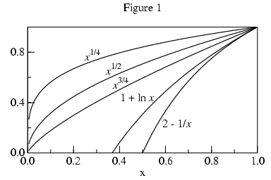
near 1, as Figure 1 shows. In fact, the slope (1/2 x-1/2) tends to infinity as
x tends to 0.
One might think that the space between successive values of
f(x) would decrease with x closing on p
when the x are evenly spaced. But that is not necessarily the
case. The square-root of 0 is 0; and that right-hand limit exists,
but the square-roots near 0 are further apart than the square-roots
near 1, as Figure 1 shows. In fact, the slope (1/2 x-1/2) tends to infinity as
x tends to 0.
Figure 1 also shows 1+ln(x) and 2-(1/x), functions whose limits at 0 tend to negative infinity. So how will the algorithm distinguish between vertical points-of-inflection and infinite limits? We will return to this question.
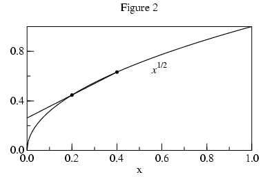 The central problem is how to find a value very close to
f(p) without actually calling f(p). With
two values of f we can construct the secant (a straight line
connecting two points on a curve) and find its intersection with
x=p. Using this extrapolated value will be more
accurate than the value of f at the sample nearest to p.
The central problem is how to find a value very close to
f(p) without actually calling f(p). With
two values of f we can construct the secant (a straight line
connecting two points on a curve) and find its intersection with
x=p. Using this extrapolated value will be more
accurate than the value of f at the sample nearest to p.
Using values of f at additional points allows us to fit higher
order curves and acheive better approximations. For n+1 points
we can fit f(x) to an nth order polynomial.
The extrapolated L values versus n are:

| ( | n | ) | (-1)k+1 |
| k |
For n=2 the fit for the forward and inverse curves (actually lines) are the same:
e0 : g(x) := a*x + b;

g(x): g(x)

e3 : eliminate([0=g(f0), 1=g(f1), 2=g(f2)], [b, a]);

e3: 0 = f0 - 2 f1 + f2
For n=3, things get more complicated.
e4 : g(x) := a*x^2 + b*x + c;

g(x): g(x)

e4 : eliminate([0=g(f0), 1=g(f1), 2=g(f2), 3=g(f3)], [c, b, a]);

            2           2        2       2                         2        2
e4: 0 = - f0  f1 + f0 f1  + (2 f0  - 3 f1 ) f2 + (- 2 f0 + 3 f1) f2  + (- f0  +

                           2     2                          2
                       2 f1  - f2 ) f3 + (f0 - 2 f1 + f2) f3
The value of f0(=L) which makes the equation true can be
determined by a root-finder; or by solving this degree 2 polynomial in
f0 using the quadratic formula.
As the degree is increased, expression size grows exponentially; quickly becoming unwieldy.
e3 : g(x) := a*x^3 + b*x^2 + c*x + d;

g(x): g(x)

e4 : eliminate([0=g(f0), 1=g(f1), 2=g(f2), 3=g(f3), 4=g(f4)], [d, c, b, a]);

                 3   2     2   3          3           3    2        2
e3:     0 = (- f0  f1  + f0  f1 ) f2 + (f0  f1 - f0 f1 ) f2  + (- f0  f1 +

           2    3        3   2       2   3          3       3    2        2
      f0 f1 ) f2  + (2 f0  f1  - 2 f0  f1  + (- 3 f0  + 4 f1 ) f2  + (3 f0  -

         2    3              3             3        3       3
     4 f1 ) f2 ) f3 + (- 2 f0  f1 + 2 f0 f1  + (3 f0  - 4 f1 ) f2 + (- 3 f0 +

              3    2        2             2          2       2
      4 f1) f2 ) f3  + (2 f0  f1 - 2 f0 f1  + (- 3 f0  + 4 f1 ) f2 + (3 f0 -

             2    3        3   2     2   3        3       3    2          2
     4 f1) f2 ) f3  + (- f0  f1  + f0  f1  + (2 f0  - 3 f1 ) f2  + (- 2 f0  +

          2    3        3       3     3    2      2       2     2    3
      3 f1 ) f2  + (- f0  + 2 f1  - f2 ) f3  + (f0  - 2 f1  + f2 ) f3 ) f4 +

          3           3          3       3                       3      3
       (f0  f1 - f0 f1  + (- 2 f0  + 3 f1 ) f2 + (2 f0 - 3 f1) f2  + (f0  -

           3     3                            3    2        2           2
       2 f1  + f2 ) f3 + (- f0 + 2 f1 - f2) f3 ) f4  + (- f0  f1 + f0 f1  +

         2       2                         2        2       2     2
    (2 f0  - 3 f1 ) f2 + (- 2 f0 + 3 f1) f2  + (- f0  + 2 f1  - f2 ) f3 + (f0 -

                                             2    3
                                2 f1 + f2) f3 ) f4
Until a more tractable form is found, the algorithm will extrapolate
from a quadratic fitted to 3 points of
f -1
when the slope tends to infinity near p.
Unfortunately, our approximation is strongly influenced by the closest f(x) sample. Using the approximation value for L in the convergence test prevents the algorithm from exiting early when the limit doesn't exist.
Although |f(x)-L| is not available, derivatives of f(x) are. Secants are proportional to the derivative of f(x). By the Mean value theorem, there is a point between the secant endpoints such that the derivative of f at that point equals the slope of the secant.
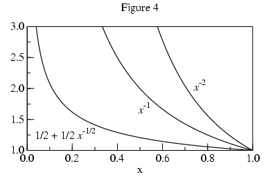 Approaching p, monotonic curves whose limit points tend to
infinity are as steep or steeper than logarithms (hyperbolic, for
example). Thus the algorithm should look for
|f'(x)| increasing proportionally faster than
|1/(x-p)| as x tends toward p. If that is
the case, then the limit is infinite. If
|f'(x)| is monotonic and increases more slowly
than |1/(x-p)| as x tends toward p, then
L is extrapolated and returned.
Approaching p, monotonic curves whose limit points tend to
infinity are as steep or steeper than logarithms (hyperbolic, for
example). Thus the algorithm should look for
|f'(x)| increasing proportionally faster than
|1/(x-p)| as x tends toward p. If that is
the case, then the limit is infinite. If
|f'(x)| is monotonic and increases more slowly
than |1/(x-p)| as x tends toward p, then
L is extrapolated and returned.
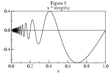 The curve sin(1/x) has no limit at 0; its derivative,
| -cos(1/x)
x2 |
Figure 5 shows a curve of x sin(pi/x), whose limit at 0 is 0. Figure 6 shows its derivative, whose envelope is pi/x.
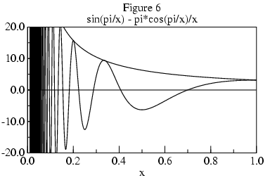
The derivative has infinitely many peaks approaching x=0. The distance between adjacent peaks and valleys is:
|
x2
x - 1 |
|
x2 sin(pi/x) - x pi cos(pi/x)
x - 1 |
|
sin(pi t)
- pi t cos(pi t)
t2 - t |
|
==== \ / ==== |
pi (-1)t
t - 1 |
While it may be possible to determine whether a limit exists from the envelope of such curves, because the magnitude of the derivative tends to infinity as x nears 0, its values are of no use in extrapolating the limit L. Apart from needing to formalize the concept of envelope, non-monotonic curves present practical problems for algorithms which will examine f at only a small number of points. If the algorithm is unlucky in its choice of points, then it will incorrectly gage the envelope. For these reasons, the algorithm is restricted to monotonic functions.
For integer j, 0 < j < n+1, let xj = p+(r j/n).
For 1 < j < n+1, let sj = f(xj) - f(xj-1).
Let hn = |sn|.
For 1 < j < n, let hj = hn n/j.
If for 1 < j < n,
|sj| =< |sj+1|,
then the limit is extrapolated from the degree n polynomial
passing through
(xj , f(xj ))
for 0 < j < n+1.
If for 1 < j < n,
|sj| > |sj+1| and
|sj| < hj,
then the limit is extrapolated from the quadratic passing through
(f(x1), x1),
(f(x2), x2), and
(f(x3), x3).
If for 1 < j < n, |sj| > |sj+1| and |sj| >= hj, then the limit tends to infinity of sign s2.
Otherwise, the limit does not exist at scale r.
For the point limits we evaluated f at a succession of evenly spaced points leading to the limit point p. Uniform spacing doesn't lead to an infinite limit point. Instead, we transform the problem by taking a point limit of g(x)=f(1/x) at 0 from 1/r.Limit of function at infinity
Suppose f(x) is a real-valued function. We can also consider the limit of function f when x increases or decreases indefinitely.
We write
lim
x -> ∞f(x) = L
if and only if
- for every ε > 0 there exists S >0 such that for all real numbers x>S, we have |f(x)-L|<ε
or we write
lim
x -> ∞f(x) = ∞
- for every R > 0 there exists S >0 such that for all real numbers x>S, we have f(x)>R.
Similarly, we can define the expressions
,
lim
x -> ∞f(x) = -∞
,
lim
x -> -∞f(x) = L
, and
lim
x -> -∞f(x) = ∞
.
lim
x -> -∞f(x) = -∞
limit procedure has been
coded in Scheme
as part of the SLIB Scheme Library.
|
I am a guest and not a member of the MIT Computer Science and Artificial Intelligence Laboratory.
My actions and comments do not reflect in any way on MIT. | ||
| agj @ alum.mit.edu | Go Figure! | |