Type Theory
Univalent Foundations of Mathematics
The Univalent Foundations Program
Institute for Advanced Study
Homotopy Type Theory
Univalent Foundations of Mathematics
The Univalent Foundations Program
Institute for Advanced Study

“Homotopy Type Theory: Univalent Foundations of Mathematics”
© 2013 The Univalent Foundations Program
Book version: first-edition-652-g5c9d883
MSC 2010 classification: 03-02, 55-02, 03B15
This work is licensed under the Creative Commons Attribution-ShareAlike 3.0 Unported License. To view a copy of this license, visit http://creativecommons.org/licenses/by-sa/3.0/.
This book is freely available at http://homotopytypetheory.org/book/.
Acknowledgment
Apart from the generous support from the Institute for Advanced Study, some contributors to the book were partially or fully supported by the following agencies and grants:
This material is based in part upon work supported by the AFOSR under the above awards. Any opinions, findings, and conclusions or recommendations expressed in this publication are those of the author(s) and do not necessarily reflect the views of the AFOSR.
This material is based in part upon work supported by the National Science Foundation under the above awards. Any opinions, findings, and conclusions or recommendations expressed in this material are those of the author(s) and do not necessarily reflect the views of the National Science Foundation.
A Special Year on Univalent Foundations of Mathematics was held in 2012-13 at the Institute for Advanced Study, School of Mathematics, organized by Steve Awodey, Thierry Coquand, and Vladimir Voevodsky. The following people were the official participants.
|
There were also the following students, whose participation was no less valuable.
|
In addition, there were the following short- and long-term visitors, including student visitors, whose contributions to the Special Year were also essential.
|
We did not set out to write a book. The present work has its origins in our collective attempts to develop a new style of “informal type theory” that can be read and understood by a human being, as a complement to a formal proof that can be checked by a machine. Univalent foundations is closely tied to the idea of a foundation of mathematics that can be implemented in a computer proof assistant. Although such a formalization is not part of this book, much of the material presented here was actually done first in the fully formalized setting inside a proof assistant, and only later “unformalized” to arrive at the presentation you find before you — a remarkable inversion of the usual state of affairs in formalized mathematics.
Each of the above-named individuals contributed something to the Special Year — and so to this book — in the form of ideas, words, or deeds. The spirit of collaboration that prevailed throughout the year was truly extraordinary.
Special thanks are due to the Institute for Advanced Study, without which this book would obviously never have come to be. It proved to be an ideal setting for the creation of this new branch of mathematics: stimulating, congenial, and supportive. May some trace of this unique atmosphere linger in the pages of this book, and in the future development of this new field of study.
The Univalent Foundations Program
Institute for Advanced Study
Princeton, April 2013
 et is a ΠW-pretopos
Homotopy type theory is a new branch of mathematics that combines aspects of several different fields in a surprising way. It is based on a recently discovered connection between homotopy theory and type theory. Homotopy theory is an outgrowth of algebraic topology and homological algebra, with relationships to higher category theory; while type theory is a branch of mathematical logic and theoretical computer science. Although the connections between the two are currently the focus of intense investigation, it is increasingly clear that they are just the beginning of a subject that will take more time and more hard work to fully understand. It touches on topics as seemingly distant as the homotopy groups of spheres, the algorithms for type checking, and the definition of weak ∞-groupoids.
Homotopy type theory also brings new ideas into the very foundation of mathematics. On the one hand, there is Voevodsky’s subtle and beautiful univalence axiom. The univalence axiom implies, in particular, that isomorphic structures can be identified, a principle that mathematicians have been happily using on workdays, despite its incompatibility with the “official” doctrines of conventional foundations. On the other hand, we have higher inductive types, which provide direct, logical descriptions of some of the basic spaces and constructions of homotopy theory: spheres, cylinders, truncations, localizations, etc. Both ideas are impossible to capture directly in classical set-theoretic foundations, but when combined in homotopy type theory, they permit an entirely new kind of “logic of homotopy types”.
This suggests a new conception of foundations of mathematics, with intrinsic homotopical content, an “invariant” conception of the objects of mathematics — and convenient machine implementations, which can serve as a practical aid to the working mathematician. This is the Univalent Foundations program. The present book is intended as a first systematic exposition of the basics of univalent foundations, and a collection of examples of this new style of reasoning — but without requiring the reader to know or learn any formal logic, or to use any computer proof assistant.
We emphasize that homotopy type theory is a young field, and univalent foundations is very much a work in progress. This book should be regarded as a “snapshot” of the state of the field at the time it was written, rather than a polished exposition of an established edifice. As we will discuss briefly later, there are many aspects of homotopy type theory that are not yet fully understood — but as of this writing, its broad outlines seem clear enough. The ultimate theory will probably not look exactly like the one described in this book, but it will surely be at least as capable and powerful; we therefore believe that univalent foundations will eventually become a viable alternative to set theory as the “implicit foundation” for the unformalized mathematics done by most mathematicians.
Type theory was originally invented by Bertrand Russell [Rus08], as a device for blocking the paradoxes in the logical foundations of mathematics that were under investigation at the time. It was later developed as a rigorous formal system in its own right (under the name “λ-calculus”) by Alonzo Church [Chu33, Chu40, Chu41]. Although it is not generally regarded as the foundation for classical mathematics, set theory being more customary, type theory still has numerous applications, especially in computer science and the theory of programming languages [Pie02]. Per Martin-Löf [ML98, ML75, ML82, ML84], among others, developed a “predicative” modification of Church’s type system, which is now usually called dependent, constructive, intuitionistic, or simply Martin-Löf type theory. This is the basis of the system that we consider here; it was originally intended as a rigorous framework for the formalization of constructive mathematics. In what follows, we will often use “type theory” to refer specifically to this system and similar ones, although type theory as a subject is much broader (see [Som10, KLN04] for the history of type theory).
In type theory, unlike set theory, objects are classified using a primitive notion of type, similar to the data-types used in programming languages. These elaborately structured types can be used to express detailed specifications of the objects classified, giving rise to principles of reasoning about these objects. To take a very simple example, the objects of a product type A×B are known to be of the form (a, b), and so one automatically knows how to construct them and how to decompose them. Similarly, an object of function type A → B can be acquired from an object of type B parametrized by objects of type A, and can be evaluated at an argument of type A. This rigidly predictable behavior of all objects (as opposed to set theory’s more liberal formation principles, allowing inhomogeneous sets) is one aspect of type theory that has led to its extensive use in verifying the correctness of computer programs. The clear reasoning principles associated with the construction of types also form the basis of modern computer proof assistants, which are used for formalizing mathematics and verifying the correctness of formalized proofs. We return to this aspect of type theory below.
One problem in understanding type theory from a mathematical point of view, however, has always been that the basic concept of type is unlike that of set in ways that have been hard to make precise. We believe that the new idea of regarding types, not as strange sets (perhaps constructed without using classical logic), but as spaces, viewed from the perspective of homotopy theory, is a significant step forward. In particular, it solves the problem of understanding how the notion of equality of elements of a type differs from that of elements of a set.
In homotopy theory one is concerned with spaces and continuous mappings between them, up to homotopy. A homotopy between a pair of continuous maps f : X → Y and g : X → Y is a continuous map H : X× [0, 1] → Y satisfying H(x, 0) = f(x) and H(x, 1) = g(x). The homotopy H may be thought of as a “continuous deformation” of f into g. The spaces X and Y are said to be homotopy equivalent, X ≃ Y, if there are continuous maps going back and forth, the composites of which are homotopical to the respective identity mappings, i.e., if they are isomorphic “up to homotopy”. Homotopy equivalent spaces have the same algebraic invariants (e.g., homology, or the fundamental group), and are said to have the same homotopy type.
Homotopy type theory (HoTT) interprets type theory from a homotopical perspective. In homotopy type theory, we regard the types as “spaces” (as studied in homotopy theory) or higher groupoids, and the logical constructions (such as the product A×B) as homotopy-invariant constructions on these spaces. In this way, we are able to manipulate spaces directly without first having to develop point-set topology (or any combinatorial replacement for it, such as the theory of simplicial sets). To briefly explain this perspective, consider first the basic concept of type theory, namely that the term a is of type A, which is written:

This expression is traditionally thought of as akin to:
“a is an element of the set A”.
However, in homotopy type theory we think of it instead as:
“a is a point of the space A”.
Similarly, every function f : A → B in type theory is regarded as a continuous map from the space A to the space B.
We should stress that these “spaces” are treated purely homotopically, not topologically. For instance, there is no notion of “open subset” of a type or of “convergence” of a sequence of elements of a type. We only have “homotopical” notions, such as paths between points and homotopies between paths, which also make sense in other models of homotopy theory (such as simplicial sets). Thus, it would be more accurate to say that we treat types as ∞-groupoids; this is a name for the “invariant objects” of homotopy theory which can be presented by topological spaces, simplicial sets, or any other model for homotopy theory. However, it is convenient to sometimes use topological words such as “space” and “path”, as long as we remember that other topological concepts are not applicable.
(It is tempting to also use the phrase homotopy type for these objects, suggesting the dual interpretation of “a type (as in type theory) viewed homotopically” and “a space considered from the point of view of homotopy theory”. The latter is a bit different from the classical meaning of “homotopy type” as an equivalence class of spaces modulo homotopy equivalence, although it does preserve the meaning of phrases such as “these two spaces have the same homotopy type”.)
The idea of interpreting types as structured objects, rather than sets, has a long pedigree, and is known to clarify various mysterious aspects of type theory. For instance, interpreting types as sheaves helps explain the intuitionistic nature of type-theoretic logic, while interpreting them as partial equivalence relations or “domains” helps explain its computational aspects. It also implies that we can use type-theoretic reasoning to study the structured objects, leading to the rich field of categorical logic. The homotopical interpretation fits this same pattern: it clarifies the nature of identity (or equality) in type theory, and allows us to use type-theoretic reasoning in the study of homotopy theory.
The key new idea of the homotopy interpretation is that the logical notion of identity a = b of two objects a, b : A of the same type A can be understood as the existence of a path p : a ↝ b from point a to point b in the space A. This also means that two functions f, g : A → B can be identified if they are homotopic, since a homotopy is just a (continuous) family of paths px : f(x) ↝ g(x) in B, one for each x : A. In type theory, for every type A there is a (formerly somewhat mysterious) type IdA of identifications of two objects of A; in homotopy type theory, this is just the path space AI of all continuous maps I → A from the unit interval. In this way, a term p : IdA(a, b) represents a path p : a ↝ b in A.
The idea of homotopy type theory arose around 2006 in independent work by Awodey and Warren [AW09] and Voevodsky [Voe06], but it was inspired by Hofmann and Streicher’s earlier groupoid interpretation [HS98]. Indeed, higher-dimensional category theory (particularly the theory of weak ∞-groupoids) is now known to be intimately connected to homotopy theory, as proposed by Grothendieck and now being studied intensely by mathematicians of both sorts. The original semantic models of Awodey–Warren and Voevodsky use well-known notions and techniques from homotopy theory which are now also in use in higher category theory, such as Quillen model categories and Kan simplicial sets.
Voevodsky recognized that the simplicial interpretation of type theory satisfies a further crucial property, dubbed univalence, which had not previously been considered in type theory (although Church’s principle of extensionality for propositions turns out to be a very special case of it). Adding univalence to type theory in the form of a new axiom has far-reaching consequences, many of which are natural, simplifying and compelling. The univalence axiom also further strengthens the homotopical view of type theory, since it holds in the simplicial model and other related models, while failing under the view of types as sets.
Very briefly, the basic idea of the univalence axiom can be explained
as follows. In type theory, one can have a universe  , the terms of
which are themselves types, A : , etc. Those types that are terms of
are commonly called small types. Like any type, has an identity
type Id
, the terms of
which are themselves types, A : , etc. Those types that are terms of
are commonly called small types. Like any type, has an identity
type Id , which expresses the identity relation A = B between small
types. Thinking of types as spaces, is a space, the points of which are
spaces; to understand its identity type, we must ask, what is a path
p : A ↝ B between spaces in ? The univalence axiom says that such paths
correspond to homotopy equivalences A ≃ B, (roughly) as explained above.
A bit more precisely, given any (small) types A and B, in addition
to the primitive type Id(A, B) of identifications of A with B, there
is the defined type Equiv(A, B) of equivalences from A to B. Since
the identity map on any object is an equivalence, there is a canonical
map,
, which expresses the identity relation A = B between small
types. Thinking of types as spaces, is a space, the points of which are
spaces; to understand its identity type, we must ask, what is a path
p : A ↝ B between spaces in ? The univalence axiom says that such paths
correspond to homotopy equivalences A ≃ B, (roughly) as explained above.
A bit more precisely, given any (small) types A and B, in addition
to the primitive type Id(A, B) of identifications of A with B, there
is the defined type Equiv(A, B) of equivalences from A to B. Since
the identity map on any object is an equivalence, there is a canonical
map,
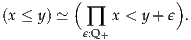
The univalence axiom states that this map is itself an equivalence. At the risk of oversimplifying, we can state this succinctly as follows:
In other words, identity is equivalent to equivalence. In particular, one may say that “equivalent types are identical”. However, this phrase is somewhat misleading, since it may sound like a sort of “skeletality” condition which collapses the notion of equivalence to coincide with identity, whereas in fact univalence is about expanding the notion of identity so as to coincide with the (unchanged) notion of equivalence.
From the homotopical point of view, univalence implies that spaces of the
same homotopy type are connected by a path in the universe , in accord
with the intuition of a classifying space for (small) spaces. From the
logical point of view, however, it is a radically new idea: it says that
isomorphic things can be identified! Mathematicians are of course used to
identifying isomorphic structures in practice, but they generally do
so by “abuse of notation”, or some other informal device, knowing
that the objects involved are not “really” identical. But in this new
foundational scheme, such structures can be formally identified, in the
logical sense that every property or construction involving one also
applies to the other. Indeed, the identification is now made explicit, and
properties and constructions can be systematically transported along it.
Moreover, the different ways in which such identifications may be
made themselves form a structure that one can (and should!) take into
account.
Thus in sum, for points A and B of the universe (i.e., small types), the
univalence axiom identifies the following three notions:
One of the classical advantages of type theory is its simple and effective techniques for working with inductively defined structures. The simplest nontrivial inductively defined structure is the natural numbers, which is inductively generated by zero and the successor function. From this statement one can algorithmically extract the principle of mathematical induction, which characterizes the natural numbers. More general inductive definitions encompass lists and well-founded trees of all sorts, each of which is characterized by a corresponding “induction principle”. This includes most data structures used in certain programming languages; hence the usefulness of type theory in formal reasoning about the latter. If conceived in a very general sense, inductive definitions also include examples such as a disjoint union A + B, which may be regarded as “inductively” generated by the two injections A → A + B and B → A + B. The “induction principle” in this case is “proof by case analysis”, which characterizes the disjoint union.
In homotopy theory, it is natural to consider also “inductively defined spaces” which are generated not merely by a collection of points, but also by collections of paths and higher paths. Classically, such spaces are called CW complexes. For instance, the circle S1 is generated by a single point and a single path from that point to itself. Similarly, the 2-sphere S2 is generated by a single point b and a single two-dimensional path from the constant path at b to itself, while the torus T2 is generated by a single point, two paths p and q from that point to itself, and a two-dimensional path from p▪q to q▪p.
By using the identification of paths with identities in homotopy type theory, these sort of “inductively defined spaces” can be characterized in type theory by “induction principles”, entirely analogously to classical examples such as the natural numbers and the disjoint union. The resulting higher inductive types give a direct “logical” way to reason about familiar spaces such as spheres, which (in combination with univalence) can be used to perform familiar arguments from homotopy theory, such as calculating homotopy groups of spheres, in a purely formal way. The resulting proofs are a marriage of classical homotopy-theoretic ideas with classical type-theoretic ones, yielding new insight into both disciplines.
Moreover, this is only the tip of the iceberg: many abstract constructions from homotopy theory, such as homotopy colimits, suspensions, Postnikov towers, localization, completion, and spectrification, can also be expressed as higher inductive types. Many of these are classically constructed using Quillen’s “small object argument”, which can be regarded as a finite way of algorithmically describing an infinite CW complex presentation of a space, just as “zero and successor” is a finite algorithmic description of the infinite set of natural numbers. Spaces produced by the small object argument are infamously complicated and difficult to understand; the type-theoretic approach is potentially much simpler, bypassing the need for any explicit construction by giving direct access to the appropriate “induction principle”. Thus, the combination of univalence and higher inductive types suggests the possibility of a revolution, of sorts, in the practice of homotopy theory.
We have claimed that univalent foundations can eventually serve as a foundation for “all” of mathematics, but so far we have discussed only homotopy theory. Of course, there are many specific examples of the use of type theory without the new homotopy type theory features to formalize mathematics, such as the recent formalization of the Feit–Thompson odd-order theorem in Coq [GAA+13].
But the traditional view is that mathematics is founded on set theory, in the sense that all mathematical objects and constructions can be coded into a theory such as Zermelo–Fraenkel set theory (ZF). However, it is well-established by now that for most mathematics outside of set theory proper, the intricate hierarchical membership structure of sets in ZF is really unnecessary: a more “structural” theory, such as Lawvere’s Elementary Theory of the Category of Sets [Law05], suffices.
In univalent foundations, the basic objects are “homotopy types” rather than sets, but we can define a class of types which behave like sets. Homotopically, these can be thought of as spaces in which every connected component is contractible, i.e. those which are homotopy equivalent to a discrete space. It is a theorem that the category of such “sets” satisfies Lawvere’s axioms (or related ones, depending on the details of the theory). Thus, any sort of mathematics that can be represented in an ETCS-like theory (which, experience suggests, is essentially all of mathematics) can equally well be represented in univalent foundations.
This supports the claim that univalent foundations is at least as good as existing foundations of mathematics. A mathematician working in univalent foundations can build structures out of sets in a familiar way, with more general homotopy types waiting in the foundational background until there is need of them. For this reason, most of the applications in this book have been chosen to be areas where univalent foundations has something new to contribute that distinguishes it from existing foundational systems.
Unsurprisingly, homotopy theory and category theory are two of these, but perhaps less obvious is that univalent foundations has something new and interesting to offer even in subjects such as set theory and real analysis. For instance, the univalence axiom allows us to identify isomorphic structures, while higher inductive types allow direct descriptions of objects by their universal properties. Thus we can generally avoid resorting to arbitrarily chosen representatives or transfinite iterative constructions. In fact, even the objects of study in ZF set theory can be characterized, inside the sets of univalent foundations, by such an inductive universal property.
One difficulty often encountered by the classical mathematician when faced with learning about type theory is that it is usually presented as a fully or partially formalized deductive system. This style, which is very useful for proof-theoretic investigations, is not particularly convenient for use in applied, informal reasoning. Nor is it even familiar to most working mathematicians, even those who might be interested in foundations of mathematics. One objective of the present work is to develop an informal style of doing mathematics in univalent foundations that is at once rigorous and precise, but is also closer to the language and style of presentation of everyday mathematics.
In present-day mathematics, one usually constructs and reasons about mathematical objects in a way that could in principle, one presumes, be formalized in a system of elementary set theory, such as ZFC — at least given enough ingenuity and patience. For the most part, one does not even need to be aware of this possibility, since it largely coincides with the condition that a proof be “fully rigorous” (in the sense that all mathematicians have come to understand intuitively through education and experience). But one does need to learn to be careful about a few aspects of “informal set theory”: the use of collections too large or inchoate to be sets; the axiom of choice and its equivalents; even (for undergraduates) the method of proof by contradiction; and so on. Adopting a new foundational system such as homotopy type theory as the implicit formal basis of informal reasoning will require adjusting some of one’s instincts and practices. The present text is intended to serve as an example of this “new kind of mathematics”, which is still informal, but could now in principle be formalized in homotopy type theory, rather than ZFC, again given enough ingenuity and patience.
It is worth emphasizing that, in this new system, such formalization can have real practical benefits. The formal system of type theory is suited to computer systems and has been implemented in existing proof assistants. A proof assistant is a computer program which guides the user in construction of a fully formal proof, only allowing valid steps of reasoning. It also provides some degree of automation, can search libraries for existing theorems, and can even extract numerical algorithms from the resulting (constructive) proofs.
We believe that this aspect of the univalent foundations program distinguishes it from other approaches to foundations, potentially providing a new practical utility for the working mathematician. Indeed, proof assistants based on older type theories have already been used to formalize substantial mathematical proofs, such as the four-color theorem and the Feit–Thompson theorem. Computer implementations of univalent foundations are presently works in progress (like the theory itself). However, even its currently available implementations (which are mostly small modifications to existing proof assistants such as Coq and Agda) have already demonstrated their worth, not only in the formalization of known proofs, but in the discovery of new ones. Indeed, many of the proofs described in this book were actually first done in a fully formalized form in a proof assistant, and are only now being “unformalized” for the first time — a reversal of the usual relation between formal and informal mathematics.
One can imagine a not-too-distant future when it will be possible for mathematicians to verify the correctness of their own papers by working within the system of univalent foundations, formalized in a proof assistant, and that doing so will become as natural as typesetting their own papers in TEX. In principle, this could be equally true for any other foundational system, but we believe it to be more practically attainable using univalent foundations, as witnessed by the present work and its formal counterpart.
One of the most striking differences between classical foundations and type theory is the idea of proof relevance, according to which mathematical statements, and even their proofs, become first-class mathematical objects. In type theory, we represent mathematical statements by types, which can be regarded simultaneously as both mathematical constructions and mathematical assertions, a conception also known as propositions as types. Accordingly, we can regard a term a : A as both an element of the type A (or in homotopy type theory, a point of the space A), and at the same time, a proof of the proposition A. To take an example, suppose we have sets A and B (discrete spaces), and consider the statement “A is isomorphic to B”. In type theory, this can be rendered as:

The logic of propositions-as-types is flexible and supports many variations, such as using only a subclass of types to represent propositions. In homotopy type theory, there are natural such subclasses arising from the fact that the system of all types, just like spaces in classical homotopy theory, is “stratified” according to the dimensions in which their higher homotopy structure exists or collapses. In particular, Voevodsky has found a purely type-theoretic definition of homotopy n-types, corresponding to spaces with no nontrivial homotopy information above dimension n. (The 0-types are the “sets” mentioned previously as satisfying Lawvere’s axioms.) Moreover, with higher inductive types, we can universally “truncate” a type into an n-type; in classical homotopy theory this would be its nth Postnikov section. Particularly important for logic is the case of homotopy (-1)-types, which we call mere propositions. Classically, every (-1)-type is empty or contractible; we interpret these possibilities as the truth values “false” and “true” respectively.
Using all types as propositions yields a “constructive” conception of logic (for more on which, see [Kol32, TvD88a, TvD88b]), which gives type theory its good computational character. For instance, every proof that something exists carries with it enough information to actually find such an object; and from a proof that “A or B” holds, one can extract either a proof that A holds or one that B holds. Thus, from every proof we can automatically extract an algorithm; this can be very useful in applications to computer programming.
However, this logic does not faithfully represent certain important classical principles of reasoning, such as the axiom of choice and the law of excluded middle. For these we need to use the “(-1)-truncated” logic, in which only the homotopy (-1)-types represent propositions; and under this interpretation, the system is fully compatible with classical mathematics. Homotopy type theory is thus compatible with both constructive and classical conceptions of logic, and many more besides.
More specifically, consider on one hand the axiom of choice: “if for every x : A there exists a y : B such that R(x, y), there is a function f : A → B such that for all x : A we have R(x, f(x)).” The pure propositions-as-types notion of “there exists” is strong enough to make this statement simply provable — yet it does not have all the consequences of the usual axiom of choice. However, in (-1)-truncated logic, this statement is not automatically true, but is a strong assumption with the same sorts of consequences as its counterpart in classical set theory.
On the other hand, consider the law of excluded middle: “for all A, either A or not A.” Interpreting this in the pure propositions-as-types logic yields a statement that is inconsistent with the univalence axiom. For since proving “A” means exhibiting an element of it, this assumption would give a uniform way of selecting an element from every nonempty type — a sort of Hilbertian choice operator. Univalence implies that the element of A selected by such a choice operator must be invariant under all self-equivalences of A, since these are identified with self-identities and every operation must respect identity; but clearly some types have automorphisms with no fixed points, e.g. we can swap the elements of a two-element type. However, the “(-1)-truncated law of excluded middle”, though also not automatically true, may consistently be assumed with most of the same consequences as in classical mathematics.
In other words, while the pure propositions-as-types logic is “constructive” in the strong algorithmic sense mentioned above, the default (-1)-truncated logic is “constructive” in a different sense (namely, that of the logic formalized by Heyting under the name “intuitionistic”); and to the latter we may freely add the axioms of choice and excluded middle to obtain a logic that may be called “classical”. Thus, the homotopical perspective reveals that classical and constructive logic can coexist, as endpoints of a spectrum of different systems, with an infinite number of possibilities in between (the homotopy n-types for -1 < n < ∞). We may speak of “LEMn” and “ACn”, with AC∞ being provable and LEM∞ inconsistent with univalence, while AC-1 and LEM-1 are the versions familiar to classical mathematicians (hence in most cases it is appropriate to assume the subscript (-1) when none is given). Indeed, one can even have useful systems in which only certain types satisfy such further “classical” principles, while types in general remain “constructive”.
It is worth emphasizing that univalent foundations does not require the use of constructive or intuitionistic logic. Most of classical mathematics which depends on the law of excluded middle and the axiom of choice can be performed in univalent foundations, simply by assuming that these two principles hold (in their proper, (-1)-truncated, form). However, type theory does encourage avoiding these principles when they are unnecessary, for several reasons.
First of all, every mathematician knows that a theorem is more powerful when proven using fewer assumptions, since it applies to more examples. The situation with AC and LEM is no different: type theory admits many interesting “nonstandard” models, such as in sheaf toposes, where classicality principles such as AC and LEM tend to fail. Homotopy type theory admits similar models in higher toposes, such as are studied in [TV02, Rez05, Lur09]. Thus, if we avoid using these principles, the theorems we prove will be valid internally to all such models.
Secondly, one of the additional virtues of type theory is its computable character. In addition to being a foundation for mathematics, type theory is a formal theory of computation, and can be treated as a powerful programming language. From this perspective, the rules of the system cannot be chosen arbitrarily the way set-theoretic axioms can: there must be a harmony between them which allows all proofs to be “executed” as programs. We do not yet fully understand the new principles introduced by homotopy type theory, such as univalence and higher inductive types, from this point of view, but the basic outlines are emerging; see, for example, [LH12]. It has been known for a long time, however, that principles such as AC and LEM are fundamentally antithetical to computability, since they assert baldly that certain things exist without giving any way to compute them. Thus, avoiding them is necessary to maintain the character of type theory as a theory of computation.
Fortunately, constructive reasoning is not as hard as it may seem. In some cases, simply by rephrasing some definitions, a theorem can be made constructive and its proof more elegant. Moreover, in univalent foundations this seems to happen more often. For instance:
Of course, these simplifications could as well be taken as evidence that the new methods will not, ultimately, prove to be really constructive. However, we emphasize again that the reader does not have to care, or worry, about constructivity in order to read this book. The point is that in all of the above examples, the version of the theory we give has independent advantages, whether or not LEM and AC are assumed to be available. Constructivity, if attained, will be an added bonus.
Given this discussion of adding new principles such as univalence, higher inductive types, AC, and LEM, one may wonder whether the resulting system remains consistent. (One of the original virtues of type theory, relative to set theory, was that it can be seen to be consistent by proof-theoretic means). As with any foundational system, consistency is a relative question: “consistent with respect to what?” The short answer is that all of the constructions and axioms considered in this book have a model in the category of Kan complexes, due to Voevodsky [KLV12] (see [LS13b] for higher inductive types). Thus, they are known to be consistent relative to ZFC (with as many inaccessible cardinals as we need nested univalent universes). Giving a more traditionally type-theoretic account of this consistency is work in progress (see, e.g., [LH12, BCH13]).
We summarize the different points of view of the type-theoretic operations in Table 1.
| Types | Logic | Sets | Homotopy | |
| A | proposition | set | space | |
| a : A | proof | element | point | |
| B(x) | predicate | family of sets | fibration | |
| b(x) : B(x) | conditional proof | family of elements | section | |
| 0, 1 | ⊥, ⊤ | ∅, {∅} | ∅, * | |
| A+ B | A∨B | disjoint union | coproduct | |
| A×B | A∧B | set of pairs | product space | |
| A →B | A ⇒B | set of functions | function space | |
| ∑(x:A) B(x) | ∃x:AB(x) | disjoint sum | total space | |
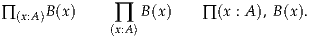
| ∏(x:A) B(x) | ∀x:AB(x) | product | space of sections | |
| IdA | equality = |  x ∈A} x ∈A} | path space AI | |
For those interested in contributing to this new branch of mathematics, it may be encouraging to know that there are many interesting open questions.
Perhaps the most pressing of them is the “constructivity” of the Univalence Axiom, posed by Voevodsky in [Voe12]. The basic system of type theory follows the structure of Gentzen’s natural deduction. Logical connectives are defined by their introduction rules, and have elimination rules justified by computation rules. Following this pattern, and using Tait’s computability method, originally designed to analyse Gödel’s Dialectica interpretation, one can show the property of normalization for type theory. This in turn implies important properties such as decidability of type-checking (a crucial property since type-checking corresponds to proof-checking, and one can argue that we should be able to “recognize a proof when we see one”), and the so-called “canonicity property” that any closed term of the type of natural numbers reduces to a numeral. This last property, and the uniform structure of introduction/elimination rules, are lost when one extends type theory with an axiom, such as the axiom of function extensionality, or the univalence axiom. Voevodsky has formulated a precise mathematical conjecture connected to this question of canonicity for type theory extended with the axiom of Univalence: given a closed term of the type of natural numbers, is it always possible to find a numeral and a proof that this term is equal to this numeral, where this proof of equality may itself use the univalence axiom? More generally, an important issue is whether it is possible to provide a constructive justification of the univalence axiom. What about if one adds other homotopically motivated constructions, like higher inductive types? These questions remain open at the present time, although methods are currently being developed to try to find answers.
Another basic issue is the difficulty of working with types, such as the natural numbers, that are essentially sets (i.e., discrete spaces), containing only trivial paths. At present, homotopy type theory can really only characterize spaces up to homotopy equivalence, which means that these “discrete spaces” may only be homotopy equivalent to discrete spaces. Type-theoretically, this means there are many paths that are equal to reflexivity, but not judgmentally equal to it (see §1.1 for the meaning of “judgmentally”). While this homotopy-invariance has advantages, these “meaningless” identity terms do introduce needless complications into arguments and constructions, so it would be convenient to have a systematic way of eliminating or collapsing them.
A more specialized, but no less important, problem is the relation between homotopy type theory and the research on higher toposes currently happening at the intersection of higher category theory and homotopy theory. There is a growing conviction among those familiar with both subjects that they are intimately connected. For instance, the notion of a univalent universe should coincide with that of an object classifier, while higher inductive types should be an “elementary” reflection of local presentability. More generally, homotopy type theory should be the “internal language” of (∞, 1)-toposes, just as intuitionistic higher-order logic is the internal language of ordinary 1-toposes. Despite this general consensus, however, details remain to be worked out — in particular, questions of coherence and strictness remain to be addressed — and doing so will undoubtedly lead to further insights into both concepts.
But by far the largest field of work to be done is in the ongoing formalization of everyday mathematics in this new system. Recent successes in formalizing some facts from basic homotopy theory and category theory have been encouraging; some of these are described in Chapters 8 and 9. Obviously, however, much work remains to be done.
The homotopy type theory community maintains a web site and group blog at http://homotopytypetheory.org, as well as a discussion email list. Newcomers are always welcome!
This book is divided into two parts. Part I, “Foundations”, develops the fundamental concepts of homotopy type theory. This is the mathematical foundation on which the development of specific subjects is built, and which is required for the understanding of the univalent foundations approach. To a programmer, this is “library code”. Since univalent foundations is a new and different kind of mathematics, its basic notions take some getting used to; thus Part I is fairly extensive.
Part II, “Mathematics”, consists of four chapters that build on the basic notions of Part I to exhibit some of the new things we can do with univalent foundations in four different areas of mathematics: homotopy theory (Chapter 8), category theory (Chapter 9), set theory (Chapter 10), and real analysis (Chapter 11). The chapters in Part II are more or less independent of each other, although occasionally one will use a lemma proven in another.
A reader who wants to seriously understand univalent foundations, and be able to work in it, will eventually have to read and understand most of Part I. However, a reader who just wants to get a taste of univalent foundations and what it can do may understandably balk at having to work through over 200 pages before getting to the “meat” in Part II. Fortunately, not all of Part I is necessary in order to read the chapters in Part II. Each chapter in Part II begins with a brief overview of its subject, what univalent foundations has to contribute to it, and the necessary background from Part I, so the courageous reader can turn immediately to the appropriate chapter for their favorite subject. For those who want to understand one or more chapters in Part II more deeply than this, but are not ready to read all of Part I, we provide here a brief summary of Part I, with remarks about which parts are necessary for which chapters in Part II.
Chapter 1 is about the basic notions of type theory, prior to any homotopical interpretation. A reader who is familiar with Martin-Löf type theory can quickly skim it to pick up the particulars of the theory we are using. However, readers without experience in type theory will need to read Chapter 1, as there are many subtle differences between type theory and other foundations such as set theory.
Chapter 2 introduces the homotopical viewpoint on type theory, along with the basic notions supporting this view, and describes the homotopical behavior of each component of the type theory from Chapter 1. It also introduces the univalence axiom (§2.10) — the first of the two basic innovations of homotopy type theory. Thus, it is quite basic and we encourage everyone to read it, especially §§2.1–2.4.
Chapter 3 describes how we represent logic in homotopy type theory, and its connection to classical logic as well as to constructive and intuitionistic logic. Here we define the law of excluded middle, the axiom of choice, and the axiom of propositional resizing (although, for the most part, we do not need to assume any of these in the rest of the book), as well as the propositional truncation which is essential for representing traditional logic. This chapter is essential background for Chapters 10 and 11, less important for Chapter 9, and not so necessary for Chapter 8.
Chapters 4 and 5 study two special topics in detail: equivalences (and related notions) and generalized inductive definitions. While these are important subjects in their own rights and provide a deeper understanding of homotopy type theory, for the most part they are not necessary for Part II. Only a few lemmas from Chapter 4 are used here and there, while the general discussions in §§5.1, 5.6 and 5.7 are helpful for providing the intuition required for Chapter 6. The generalized sorts of inductive definition discussed in §5.7 are also used in a few places in Chapters 10 and 11.
Chapter 6 introduces the second basic innovation of homotopy type theory — higher inductive types — with many examples. Higher inductive types are the primary object of study in Chapter 8, and some particular ones play important roles in Chapters 10 and 11. They are not so necessary for Chapter 9, although one example is used in §9.9.
Finally, Chapter 7 discusses homotopy n-types and related notions such as n-connected types. These notions are important for Chapter 8, but not so important in the rest of Part II, although the case n = -1 of some of the lemmas are used in §10.1.
This completes Part I. As mentioned above, Part II consists of four largely unrelated chapters, each describing what univalent foundations has to offer to a particular subject.
Of the chapters in Part II, Chapter 8 (Homotopy theory) is perhaps the most radical. Univalent foundations has a very different “synthetic” approach to homotopy theory in which homotopy types are the basic objects (namely, the types) rather than being constructed using topological spaces or some other set-theoretic model. This enables new styles of proof for classical theorems in algebraic topology, of which we present a sampling, from π1(S1) = Z to the Freudenthal suspension theorem.
In Chapter 9 (Category theory), we develop some basic (1-)category theory, adhering to the principle of the univalence axiom that equality is isomorphism. This has the pleasant effect of ensuring that all definitions and constructions are automatically invariant under equivalence of categories: indeed, equivalent categories are equal just as equivalent types are equal. (It also has connections to higher category theory and higher topos theory.)
Chapter 10 (Set theory) studies sets in univalent foundations. The category of sets has its usual properties, hence provides a foundation for any mathematics that doesn’t need homotopical or higher-categorical structures. We also observe that univalence makes cardinal and ordinal numbers a bit more pleasant, and that higher inductive types yield a cumulative hierarchy satisfying the usual axioms of Zermelo–Fraenkel set theory.
In Chapter 11 (Real numbers), we summarize the construction of Dedekind real numbers, and then observe that higher inductive types allow a definition of Cauchy real numbers that avoids some associated problems in constructive mathematics. Then we sketch a similar approach to Conway’s surreal numbers.
Each chapter in this book ends with a Notes section, which collects historical comments, references to the literature, and attributions of results, to the extent possible. We have also included Exercises at the end of each chapter, to assist the reader in gaining familiarity with doing mathematics in univalent foundations.
Finally, recall that this book was written as a massively collaborative effort by a large number of people. We have done our best to achieve consistency in terminology and notation, and to put the mathematics in a linear sequence that flows logically, but it is very likely that some imperfections remain. We ask the reader’s forgiveness for any such infelicities, and welcome suggestions for improvement of the next edition. Part I Foundations
Homotopy type theory is (among other things) a foundational language for mathematics, i.e., an alternative to Zermelo–Fraenkel set theory. However, it behaves differently from set theory in several important ways, and that can take some getting used to. Explaining these differences carefully requires us to be more formal here than we will be in the rest of the book. As stated in the introduction, our goal is to write type theory informally; but for a mathematician accustomed to set theory, more precision at the beginning can help avoid some common misconceptions and mistakes.
We note that a set-theoretic foundation has two “layers”: the deductive system of first-order logic, and, formulated inside this system, the axioms of a particular theory, such as ZFC. Thus, set theory is not only about sets, but rather about the interplay between sets (the objects of the second layer) and propositions (the objects of the first layer).
By contrast, type theory is its own deductive system: it need not be formulated inside any superstructure, such as first-order logic. Instead of the two basic notions of set theory, sets and propositions, type theory has one basic notion: types. Propositions (statements which we can prove, disprove, assume, negate, and so on1 ) are identified with particular types, via the correspondence shown in Table 1 on page 18. Thus, the mathematical activity of proving a theorem is identified with a special case of the mathematical activity of constructing an object—in this case, an inhabitant of a type that represents a proposition.
This leads us to another difference between type theory and set theory, but to explain it we must say a little about deductive systems in general. Informally, a deductive system is a collection of rules for deriving things called judgments. If we think of a deductive system as a formal game, then the judgments are the “positions” in the game which we reach by following the game rules. We can also think of a deductive system as a sort of algebraic theory, in which case the judgments are the elements (like the elements of a group) and the deductive rules are the operations (like the group multiplication). From a logical point of view, the judgments can be considered to be the “external” statements, living in the metatheory, as opposed to the “internal” statements of the theory itself.
In the deductive system of first-order logic (on which set theory is based), there is only one kind of judgment: that a given proposition has a proof. That is, each proposition A gives rise to a judgment “A has a proof”, and all judgments are of this form. A rule of first-order logic such as “from A and B infer A∧B” is actually a rule of “proof construction” which says that given the judgments “A has a proof” and “B has a proof”, we may deduce that “A∧B has a proof”. Note that the judgment “A has a proof” exists at a different level from the proposition A itself, which is an internal statement of the theory.
The basic judgment of type theory, analogous to “A has a proof”, is written “a : A” and pronounced as “the term a has type A”, or more loosely “a is an element of A” (or, in homotopy type theory, “a is a point of A”). When A is a type representing a proposition, then a may be called a witness to the provability of A, or evidence of the truth of A (or even a proof of A, but we will try to avoid this confusing terminology). In this case, the judgment a : A is derivable in type theory (for some a) precisely when the analogous judgment “A has a proof” is derivable in first-order logic (modulo differences in the axioms assumed and in the encoding of mathematics, as we will discuss throughout the book).
On the other hand, if the type A is being treated more like a set than like a proposition (although as we will see, the distinction can become blurry), then “a : A” may be regarded as analogous to the set-theoretic statement “a ∈ A”. However, there is an essential difference in that “a : A” is a judgment whereas “a ∈ A” is a proposition. In particular, when working internally in type theory, we cannot make statements such as “if a : A then it is not the case that b : B”, nor can we “disprove” the judgment “a : A”.
A good way to think about this is that in set theory, “membership” is a relation which may or may not hold between two pre-existing objects “a” and “A”, while in type theory we cannot talk about an element “a” in isolation: every element by its very nature is an element of some type, and that type is (generally speaking) uniquely determined. Thus, when we say informally “let x be a natural number”, in set theory this is shorthand for “let x be a thing and assume that x ∈N”, whereas in type theory “let x : N” is an atomic statement: we cannot introduce a variable without specifying its type.
At first glance, this may seem an uncomfortable restriction, but it is arguably closer to the intuitive mathematical meaning of “let x be a natural number”. In practice, it seems that whenever we actually need “a ∈ A” to be a proposition rather than a judgment, there is always an ambient set B of which a is known to be an element and A is known to be a subset. This situation is also easy to represent in type theory, by taking a to be an element of the type B, and A to be a predicate on B; see §3.5.
A last difference between type theory and set theory is the treatment of equality. The familiar notion of equality in mathematics is a proposition: e.g. we can disprove an equality or assume an equality as a hypothesis. Since in type theory, propositions are types, this means that equality is a type: for elements a, b : A (that is, both a : A and b : A) we have a type “a =A b”. (In homotopy type theory, of course, this equality proposition can behave in unfamiliar ways: see §1.12 and Chapter 2, and the rest of the book). When a =A b is inhabited, we say that a and b are (propositionally) equal.
However, in type theory there is also a need for an equality judgment, existing at the same level as the judgment “x : A”. This is called judgmental equality or definitional equality, and we write it as a ≡ b : A or simply a ≡ b. It is helpful to think of this as meaning “equal by definition”. For instance, if we define a function f : N →N by the equation f(x) = x2, then the expression f(3) is equal to 32 by definition. Inside the theory, it does not make sense to negate or assume an equality-by-definition; we cannot say “if x is equal to y by definition, then z is not equal to w by definition”. Whether or not two expressions are equal by definition is just a matter of expanding out the definitions; in particular, it is algorithmically decidable (though the algorithm is necessarily meta-theoretic, not internal to the theory).
As type theory becomes more complicated, judgmental equality can get more subtle than this, but it is a good intuition to start from. Alternatively, if we regard a deductive system as an algebraic theory, then judgmental equality is simply the equality in that theory, analogous to the equality between elements of a group—the only potential for confusion is that there is also an object inside the deductive system of type theory (namely the type “a = b”) which behaves internally as a notion of “equality”.
The reason we want a judgmental notion of equality is so that it can control the other form of judgment, “a : A”. For instance, suppose we have given a proof that 32 = 9, i.e. we have derived the judgment p : (32 = 9) for some p. Then the same witness p ought to count as a proof that f(3) = 9, since f(3) is 32 by definition. The best way to represent this is with a rule saying that given the judgments a : A and A ≡ B, we may derive the judgment a : B.
Thus, for us, type theory will be a deductive system based on two forms of judgment:
| Judgment | Meaning |
| a : A | “a is an object of type A” |
| a ≡ b : A | “a and b are definitionally equal objects of type A” |
When introducing a definitional equality, i.e., defining one thing to be equal to another, we will use the symbol “:≡”. Thus, the above definition of the function f would be written as f(x) :≡ x2.
Because judgments cannot be put together into more complicated statements, the symbols “:” and “≡” bind more loosely than anything else.2 Thus, for instance, “p : x = y” should be parsed as “p : (x = y)”, which makes sense since “x = y” is a type, and not as “(p : x) = y”, which is senseless since “p : x” is a judgment and cannot be equal to anything. Similarly, “A ≡ x = y” can only be parsed as “A ≡ (x = y)”, although in extreme cases such as this, one ought to add parentheses anyway to aid reading comprehension. Moreover, later on we will fall into the common notation of chaining together equalities — e.g. writing a = b = c = d to mean “a = b and b = c and c = d, hence a = d” — and we will also include judgmental equalities in such chains. Context usually suffices to make the intent clear.
This is perhaps also an appropriate place to mention that the common mathematical notation “f : A → B”, expressing the fact that f is a function from A to B, can be regarded as a typing judgment, since we use “A → B” as notation for the type of functions from A to B (as is standard practice in type theory; see §1.4).
Judgments may depend on assumptions of the form x : A, where x is a variable and A is a type. For example, we may construct an object m + n : N under the assumptions that m, n : N. Another example is that assuming A is a type, x, y : A, and p : x =A y, we may construct an element p-1 : y =A x. The collection of all such assumptions is called the context; from a topological point of view it may be thought of as a “parameter space”. In fact, technically the context must be an ordered list of assumptions, since later assumptions may depend on previous ones: the assumption x : A can only be made after the assumptions of any variables appearing in the type A.
If the type A in an assumption x : A represents a proposition, then the assumption is a type-theoretic version of a hypothesis: we assume that the proposition A holds. When types are regarded as propositions, we may omit the names of their proofs. Thus, in the second example above we may instead say that assuming x =A y, we can prove y =A x. However, since we are doing “proof-relevant” mathematics, we will frequently refer back to proofs as objects. In the example above, for instance, we may want to establish that p-1 together with the proofs of transitivity and reflexivity behave like a groupoid; see Chapter 2.
Note that under this meaning of the word assumption, we can assume a propositional equality (by assuming a variable p : x = y), but we cannot assume a judgmental equality x ≡ y, since it is not a type that can have an element. However, we can do something else which looks kind of like assuming a judgmental equality: if we have a type or an element which involves a variable x : A, then we can substitute any particular element a : A for x to obtain a more specific type or element. We will sometimes use language like “now assume x ≡ a” to refer to this process of substitution, even though it is not an assumption in the technical sense introduced above.
By the same token, we cannot prove a judgmental equality either, since it is not a type in which we can exhibit a witness. Nevertheless, we will sometimes state judgmental equalities as part of a theorem, e.g. “there exists f : A → B such that f(x) ≡ y”. This should be regarded as the making of two separate judgments: first we make the judgment f : A → B for some element f, then we make the additional judgment that f(x) ≡ y.
In the rest of this chapter, we attempt to give an informal presentation of type theory, sufficient for the purposes of this book; we give a more formal account in Appendix A. Aside from some fairly obvious rules (such as the fact that judgmentally equal things can always be substituted for each other), the rules of type theory can be grouped into type formers. Each type former consists of a way to construct types (possibly making use of previously constructed types), together with rules for the construction and behavior of elements of that type. In most cases, these rules follow a fairly predictable pattern, but we will not attempt to make this precise here; see however the beginning of §1.5 and also Chapter 5.
An important aspect of the type theory presented in this chapter is that it consists entirely of rules, without any axioms. In the description of deductive systems in terms of judgments, the rules are what allow us to conclude one judgment from a collection of others, while the axioms are the judgments we are given at the outset. If we think of a deductive system as a formal game, then the rules are the rules of the game, while the axioms are the starting position. And if we think of a deductive system as an algebraic theory, then the rules are the operations of the theory, while the axioms are the generators for some particular free model of that theory.
In set theory, the only rules are the rules of first-order logic (such as the rule allowing us to deduce “A∧B has a proof” from “A has a proof” and “B has a proof”): all the information about the behavior of sets is contained in the axioms. By contrast, in type theory, it is usually the rules which contain all the information, with no axioms being necessary. For instance, in §1.5 we will see that there is a rule allowing us to deduce the judgment “(a, b) : A×B” from “a : A” and “b : B”, whereas in set theory the analogous statement would be (a consequence of) the pairing axiom.
The advantage of formulating type theory using only rules is that rules are “procedural”. In particular, this property is what makes possible (though it does not automatically ensure) the good computational properties of type theory, such as “canonicity”. However, while this style works for traditional type theories, we do not yet understand how to formulate everything we need for homotopy type theory in this way. In particular, in §§2.9 and 2.10 and Chapter 6 we will have to augment the rules of type theory presented in this chapter by introducing additional axioms, notably the univalence axiom. In this chapter, however, we confine ourselves to a traditional rule-based type theory.
Given types A and B, we can construct the type A → B of functions with domain A and codomain B. We also sometimes refer to functions as maps. Unlike in set theory, functions are not defined as functional relations; rather they are a primitive concept in type theory. We explain the function type by prescribing what we can do with functions, how to construct them and what equalities they induce.
Given a function f : A → B and an element of the domain a : A, we can apply the function to obtain an element of the codomain B, denoted f(a) and called the value of f at a. It is common in type theory to omit the parentheses and denote f(a) simply by fa, and we will sometimes do this as well.
But how can we construct elements of A → B? There are two equivalent ways: either by direct definition or by using λ-abstraction. Introducing a function by definition means that we introduce a function by giving it a name — let’s say, f — and saying we define f : A → B by giving an equation
 | (1.2.1) |
where x is a variable and Φ is an expression which may use x. In order for this to be valid, we have to check that Φ : B assuming x : A.
Now we can compute f(a) by replacing the variable x in Φ with a. As an example, consider the function f : N →N which is defined by f(x) :≡ x + x. (We will define N and + in §1.9.) Then f(2) is judgmentally equal to 2 + 2.
If we don’t want to introduce a name for the function, we can use λ-abstraction. Given an expression Φ of type B which may use x : A, as above, we write λ(x:A).Φ to indicate the same function defined by (1.2.1). Thus, we have
For the example in the previous paragraph, we have the typing judgment
As another example, for any types A and B and any element y : B, we have a constant function (λ(x:A).y) : A → B.
We generally omit the type of the variable x in a λ-abstraction and write λx.Φ, since the typing x : A is inferable from the judgment that the function λx.Φ has type A → B. By convention, the “scope” of the variable binding “λx.” is the entire rest of the expression, unless delimited with parentheses. Thus, for instance, λx.x + x should be parsed as λx.(x + x), not as (λx.x) + x (which would, in this case, be ill-typed anyway).
Another equivalent notation is
We may also sometimes use a blank “–” in the expression Φ in place of a variable, to denote an implicit λ-abstraction. For instance, g(x, –) is another way to write λy.g(x, y).
Now a λ-abstraction is a function, so we can apply it to an argument a : A. We then have the following computation rule3 , which is a definitional equality:
where Φ′ is the expression Φ in which all occurrences of x have been replaced by a. Continuing the above example, we have
Note that from any function f : A → B, we can construct a lambda abstraction function λx.f(x). Since this is by definition “the function that applies f to its argument” we consider it to be definitionally equal to f:4
This equality is the uniqueness principle for function types, because it shows that f is uniquely determined by its values.
The introduction of functions by definitions with explicit parameters can be reduced to simple definitions by using λ-abstraction: i.e., we can read a definition of f : A → B by

as

When doing calculations involving variables, we have to be careful when replacing a variable with an expression that also involves variables, because we want to preserve the binding structure of expressions. By the binding structure we mean the invisible link generated by binders such as λ, Π and Σ (the latter we are going to meet soon) between the place where the variable is introduced and where it is used. As an example, consider f : N → (N →N) defined as
Now if we have assumed somewhere that y : N, then what is f(y)? It would be wrong to just naively replace x by y everywhere in the expression “λy.x + y” defining f(x), obtaining λy.y + y, because this means that y gets captured. Previously, the substituted y was referring to our assumption, but now it is referring to the argument of the λ-abstraction. Hence, this naive substitution would destroy the binding structure, allowing us to perform calculations which are semantically unsound.
But what is f(y) in this example? Note that bound (or “dummy”) variables such as y in the expression λy.x + y have only a local meaning, and can be consistently replaced by any other variable, preserving the binding structure. Indeed, λy.x + y is declared to be judgmentally equal5 to λz.x + z. It follows that f(y) is judgmentally equal to λz.y + z, and that answers our question. (Instead of z, any variable distinct from y could have been used, yielding an equal result.)
Of course, this should all be familiar to any mathematician: it is the same
phenomenon as the fact that if f(x) :≡∫
12 , then f(t) is not ∫
12
, then f(t) is not ∫
12 but
rather ∫
12
but
rather ∫
12 . A λ-abstraction binds a dummy variable in exactly the same
way that an integral does.
. A λ-abstraction binds a dummy variable in exactly the same
way that an integral does.
We have seen how to define functions in one variable. One way to define functions in several variables would be to use the cartesian product, which will be introduced later; a function with parameters A and B and results in C would be given the type f : A×B → C. However, there is another choice that avoids using product types, which is called currying (after the mathematician Haskell Curry).
The idea of currying is to represent a function of two inputs a : A and b : B as a function which takes one input a : A and returns another function, which then takes a second input b : B and returns the result. That is, we consider two-variable functions to belong to an iterated function type, f : A → (B → C). We may also write this without the parentheses, as f : A → B → C, with associativity to the right as the default convention. Then given a : A and b : B, we can apply f to a and then apply the result to b, obtaining f(a)(b) : C. To avoid the proliferation of parentheses, we allow ourselves to write f(a)(b) as f(a, b) even though there are no products involved. When omitting parentheses around function arguments entirely, we write fab for (fa)b, with the default associativity now being to the left so that f is applied to its arguments in the correct order.
Our notation for definitions with explicit parameters extends to this situation: we can define a named function f : A → B → C by giving an equation

where Φ : C assuming x : A and y : B. Using λ-abstraction this corresponds to

which may also be written as
We can also implicitly abstract over multiple variables by writing multiple blanks, e.g. g(–, –) means λx.λy.g(x, y). Currying a function of three or more arguments is a straightforward extension of what we have just described.
So far, we have been using the expression “A is a type” informally. We are
going to make this more precise by introducing universes. A universe is a
type whose elements are types. As in naive set theory, we might wish for a
universe of all types ∞ including itself (that is, with ∞ : ∞). However, as
in set theory, this is unsound, i.e. we can deduce from it that every type,
including the empty type representing the proposition False (see §1.7), is
inhabited. For instance, using a representation of sets as trees, we can directly
encode Russell’s paradox [Coq92].
To avoid the paradox we introduce a hierarchy of universes
where every universe i is an element of the next universe i+1. Moreover,
we assume that our universes are cumulative, that is that all the elements of
the ith universe are also elements of the (i + 1)st universe, i.e. if A : i then
also A : i+1. This is convenient, but has the slightly unpleasant consequence
that elements no longer have unique types, and is a bit tricky in other ways
that need not concern us here; see the Notes.
When we say that A is a type, we mean that it inhabits some universe i.
We usually want to avoid mentioning the level i explicitly, and just assume
that levels can be assigned in a consistent way; thus we may write A :
omitting the level. This way we can even write : , which can be
read as i : i+1, having left the indices implicit. Writing universes in
this style is referred to as typical ambiguity. It is convenient but a
bit dangerous, since it allows us to write valid-looking proofs that
reproduce the paradoxes of self-reference. If there is any doubt about
whether an argument is correct, the way to check it is to try to assign
levels consistently to all universes appearing in it. When some universe
is assumed, we may refer to types belonging to as small types.
To model a collection of types varying over a given type A, we use
functions B : A → whose codomain is a universe. These functions are called
families of types (or sometimes dependent types); they correspond to families
of sets as used in set theory.
An example of a type family is the family of finite sets Fin : N →, where
Fin(n) is a type with exactly n elements. (We cannot define the family Fin yet —
indeed, we have not even introduced its domain N yet — but we will be able
to soon; see Exercise 1.9.) We may denote the elements of Fin(n) by
0n, 1n, …, (n- 1)n, with subscripts to emphasize that the elements of Fin(n) are
different from those of Fin(m) if n is different from m, and all are different
from the ordinary natural numbers (which we will introduce in §1.9).
A more trivial (but very important) example of a type family is the
constant type family at a type B : , which is of course the constant function
(λ(x:A).B) : A →.
As a non-example, in our version of type theory there is no type family
“λ(i:N).i”. Indeed, there is no universe large enough to be its codomain.
Moreover, we do not even identify the indices i of the universes i with
the natural numbers N of type theory (the latter to be introduced in
§1.9).
In type theory we often use a more general version of function types, called a Π-type or dependent function type. The elements of a Π-type are functions whose codomain type can vary depending on the element of the domain to which the function is applied, called dependent functions. The name “Π-type” is used because this type can also be regarded as the cartesian product over a given type.
Given a type A : and a family B : A →, we may construct the type of
dependent functions ∏(x:A) B(x) : . There are many alternative notations for
this type, such as
If B is a constant family, then the dependent product type is the ordinary function type:
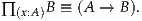
Indeed, all the constructions of Π-types are generalizations of the corresponding constructions on ordinary function types.
We can introduce dependent functions by explicit definitions: to define f : ∏(x:A) B(x), where f is the name of a dependent function to be defined, we need an expression Φ : B(x) possibly involving the variable x : A, and we write
Alternatively, we can use λ-abstraction
 | (1.4.1) |
As with non-dependent functions, we can apply a dependent function f : ∏(x:A) B(x) to an argument a : A to obtain an element f(a) : B(a). The equalities are the same as for the ordinary function type, i.e. we have the computation rule given a : A we have f(a) ≡ Φ′ and (λx.Φ)(a) ≡ Φ′, where Φ′ is obtained by replacing all occurrences of x in Φ by a (avoiding variable capture, as always). Similarly, we have the uniqueness principle f ≡ (λx.f(x)) for any f : ∏(x:A) B(x).
As an example, recall from §1.3 that there is a type family Fin : N → whose
values are the standard finite sets, with elements 0n, 1n, …, (n- 1)n : Fin(n).
There is then a dependent function fmax : ∏(n:N) Fin(n + 1) which returns the
“largest” element of each nonempty finite type, fmax(n) :≡ nn+1. As was the
case for Fin itself, we cannot define fmax yet, but we will be able to soon; see
Exercise 1.9.
Another important class of dependent function types, which we can define
now, are functions which are polymorphic over a given universe. A
polymorphic function is one which takes a type as one of its arguments, and
then acts on elements of that type (or other types constructed from it). An
example is the polymorphic identity function id : ∏(A:) A → A, which we
define by id :≡ λ(A:).λ(x:A).x.
We sometimes write some arguments of a dependent function as subscripts. For instance, we might equivalently define the polymorphic identity function by idA(x) :≡ x. Moreover, if an argument can be inferred from context, we may omit it altogether. For instance, if a : A, then writing id(a) is unambiguous, since id must mean idA in order for it to be applicable to a.
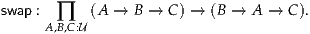
Another, less trivial, example of a polymorphic function is the “swap” operation that switches the order of the arguments of a (curried) two-argument function:
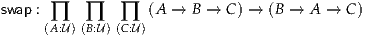
We can define this by

We might also equivalently write the type arguments as subscripts:
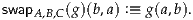 " class="math-display" >
Note that as we did for ordinary functions, we use currying to define
dependent functions with several arguments (such as swap). However, in the
dependent case the second domain may depend on the first one, and
the codomain may depend on both. That is, given A : and type
families B : A → and C : ∏(x:A) B(x) →, we may construct the
type ∏(x:A) ∏(y:B(x)) C(x, y) of functions with two arguments. (Like
λ-abstractions, Πs automatically scope over the rest of the expression unless
delimited; thus C : ∏(x:A) B(x) → means C : ∏(x:A) (B(x) →).) In the
case when B is constant and equal to A, we may condense the notation and
write ∏(x,y:A) ; for instance, the type of swap could also be written
as
Finally, given f : ∏(x:A) ∏(y:B(x)) C(x, y) and arguments a : A and b : B(a), we have f(a)(b) : C(a, b), which, as before, we write as f(a, b) : C(a, b).
Given types A, B : we introduce the type A×B : , which we call their
cartesian product. We also introduce a nullary product type, called the unit
type 1 : . We intend the elements of A×B to be pairs (a, b) : A×B, where
a : A and b : B, and the only element of 1 to be some particular object ⋆ : 1.
However, unlike in set theory, where we define ordered pairs to be
particular sets and then collect them all together into the cartesian
product, in type theory, ordered pairs are a primitive concept, as are
functions.
Remark 1.5.1. There is a general pattern for introduction of a new kind of type in type theory, and because products are our second example following this pattern,6 it is worth emphasizing the general form: To specify a type, we specify:
When the uniqueness principle is not taken as a rule of judgmental equality, it is often nevertheless provable as a propositional equality from the other rules for the type. In this case we call it a propositional uniqueness principle. (In later chapters we will also occasionally encounter propositional computation rules.)
The inference rules in Appendix A.2 are organized and named accordingly; see, for example, Appendix A.2.4, where each possibility is realized.
The way to construct pairs is obvious: given a : A and b : B, we may form (a, b) : A×B. Similarly, there is a unique way to construct elements of 1, namely we have ⋆ : 1. We expect that “every element of A×B is a pair”, which is the uniqueness principle for products; we do not assert this as a rule of type theory, but we will prove it later on as a propositional equality.
Now, how can we use pairs, i.e. how can we define functions out of a product type? Let us first consider the definition of a non-dependent function f : A×B → C. Since we intend the only elements of A×B to be pairs, we expect to be able to define such a function by prescribing the result when f is applied to a pair (a, b). We can prescribe these results by providing a function g : A → B → C. Thus, we introduce a new rule (the elimination rule for products), which says that for any such g, we can define a function f : A×B → C by
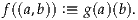
We avoid writing g(a, b) here, in order to emphasize that g is not a function on a product. (However, later on in the book we will often write g(a, b) both for functions on a product and for curried functions of two variables.) This defining equation is the computation rule for product types.
Note that in set theory, we would justify the above definition of f by the fact that every element of A×B is a pair, so that it suffices to define f on pairs. By contrast, type theory reverses the situation: we assume that a function on A×B is well-defined as soon as we specify its values on tuples, and from this (or more precisely, from its more general version for dependent functions, below) we will be able to prove that every element of A×B is a pair. From a category-theoretic perspective, we can say that we define the product A×B to be left adjoint to the “exponential” B → C, which we have already introduced.
As an example, we can derive the projection functions
| pr1 | : A×B → A | ||
| pr2 | : A×B → B |
| pr1((a, b)) | :≡ a | ||
| pr2((a, b)) | :≡ b. |
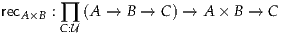 | (1.5.2) |
with the defining equation

Then instead of defining functions such as pr1 and pr2 directly by a defining equation, we could define
| pr1 | :≡recA×B(A, λa.λb.a) | ||
| pr2 | :≡recA×B(B, λa.λb.b). |
We leave it as a simple exercise to show that the recursor can be derived from the projections and vice versa.
We also have a recursor for the unit type:
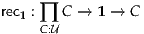
with the defining equation
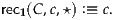
Although we include it to maintain the pattern of type definitions, the recursor for 1 is completely useless, because we could have defined such a function directly by simply ignoring the argument of type 1.
To be able to define dependent functions over the product type, we have to
generalize the recursor. Given C : A×B →, we may define a function
f : ∏(x:A×B) C(x) by providing a function
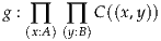 |
with defining equation
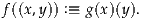
For example, in this way we can prove the propositional uniqueness principle, which says that every element of A×B is equal to a pair. Specifically, we can construct a function
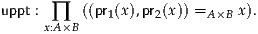
Here we are using the identity type, which we are going to introduce below in §1.12. However, all we need to know now is that there is a reflexivity element reflx : x =A x for any x : A. Given this, we can define
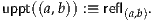
This construction works, because in the case that x :≡ (a, b) we can calculate

using the defining equations for the projections. Therefore,

is well-typed, since both sides of the equality are judgmentally equal.
More generally, the ability to define dependent functions in this way
means that to prove a property for all elements of a product, it is enough
to prove it for its canonical elements, the tuples. When we come to
inductive types such as the natural numbers, the analogous property will
be the ability to write proofs by induction. Thus, if we do as we did
above and apply this principle once in the universal case, we call the
resulting function induction for product types: given A, B : we have
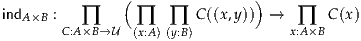
with the defining equation

Similarly, we may speak of a dependent function defined on pairs being obtained from the induction principle of the cartesian product. It is easy to see that the recursor is just the special case of induction in the case that the family C is constant. Because induction describes how to use an element of the product type, induction is also called the (dependent) eliminator, and recursion the non-dependent eliminator.
Induction for the unit type turns out to be more useful than the recursor:
with the defining equation
Induction enables us to prove the propositional uniqueness principle for 1, which asserts that its only inhabitant is ⋆. That is, we can construct
by using the defining equations
or equivalently by using induction:

Just as we generalized function types (§1.2) to dependent function types (§1.4), it is often useful to generalize the product types from §1.5 to allow the type of the second component of a pair to vary depending on the choice of the first component. This is called a dependent pair type, or Σ-type, because in set theory it corresponds to an indexed sum (in the sense of coproduct or disjoint union) over a given type.
Given a type A : and a family B : A →, the dependent pair type is
written as ∑(x:A) B(x) : . Alternative notations are

Like other binding constructs such as λ-abstractions and Πs, Σs automatically scope over the rest of the expression unless delimited, so e.g. ∑(x:A) B(x) ×C(x) means ∑(x:A) (B(x) ×C(x)).
The way to construct elements of a dependent pair type is by pairing: we have (a, b) : ∑(x:A) B(x) given a : A and b : B(a). If B is constant, then the dependent pair type is the ordinary cartesian product type:
All the constructions on Σ-types arise as straightforward generalizations of the ones for product types, with dependent functions often replacing non-dependent ones.
For instance, the recursion principle says that to define a non-dependent function out of a Σ-type f : ( ∑(x:A) B(x)) → C, we provide a function g : ∏(x:A) B(x) → C, and then we can define f via the defining equation
For instance, we can derive the first projection from a Σ-type:
 |
by the defining equation
 |
However, since the type of the second component of a pair
 |
is B(a), the second projection must be a dependent function, whose type involves the first projection function:
Thus we need the induction principle for Σ-types (the “dependent
eliminator”). This says that to construct a dependent function out of a Σ-type
into a family C : ( ∑(x:A) B(x)) →, we need a function
We can then derive a function
Applying this with C(p) :≡ B(pr1(p)), we can define
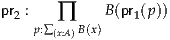 |
with the obvious equation
To convince ourselves that this is correct, we note that B(pr1((a, b))) ≡ B(a), using the defining equation for pr1, and indeed b : B(a).
We can package the recursion and induction principles into the recursor for Σ:

with the defining equation
and the corresponding induction operator:
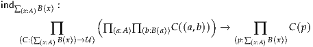
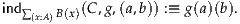
As before, the recursor is the special case of induction when the family C is constant.
As a further example, consider the following principle, where A and B are
types and R : A → B →.

We may regard R as a “proof-relevant relation” between A and B, with R(a, b) the type of witnesses for relatedness of a : A and b : B. Then ac says intuitively that if we have a dependent function g assigning to every a : A a dependent pair (b, r) where b : B and r : R(a, b), then we have a function f : A → B and a dependent function assigning to every a : A a witness that R(a, f(a)). Our intuition tells us that we can just split up the values of g into their components. Indeed, using the projections we have just defined, we can define:
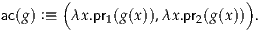
To verify that this is well-typed, note that if g : ∏(x:A) ∑(y:B) R(x, y), we have
| λx.pr1(g(x)) | : A → B, | ||
| λx.pr2(g(x)) | : ∏(x:A)R(x, pr1(g(x))). |

Thus, we have

as required.
If we read Π as “for all” and Σ as “there exists”, then the type of the function ac expresses: if for all x : Athere is a y : B such that R(x, y), then there is a function f : A → B such that for all x : Awe have R(x, f(x)). Since this sounds like a version of the axiom of choice, the function ac has traditionally been called the type-theoretic axiom of choice, and as we have just shown, it can be proved directly from the rules of type theory, rather than having to be taken as an axiom. However, note that no choice is actually involved, since the choices have already been given to us in the premise: all we have to do is take it apart into two functions: one representing the choice and the other its correctness. In §3.8 we will give another formulation of an “axiom of choice” which is closer to the usual one.
Dependent pair types are often used to define types of mathematical
structures, which commonly consist of several dependent pieces of data. To
take a simple example, suppose we want to define a magma to be a type A
together with a binary operation m : A → A → A. The precise meaning of the
phrase “together with” (and the synonymous “equipped with”) is that “a
magma” is a pair (A, m) consisting of a type A : and an operation
m : A → A → A. Since the type A → A → A of the second component m of
this pair depends on its first component A, such pairs belong to a dependent
pair type. Thus, the definition “a magma is a type A together with a binary
operation m : A → A → A” should be read as defining the type of magmas to
be
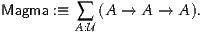
Given a magma, we extract its underlying type (its “carrier”) with the first projection pr1, and its operation with the second projection pr2. Of course, structures built from more than two pieces of data require iterated pair types, which may be only partially dependent; for instance the type of pointed magmas (magmas (A, m) equipped with a basepoint e : A) is
 " class="math-display" >
We generally also want to impose axioms on such a structure, e.g. to make a pointed magma into a monoid or a group. This can also be done using Σ-types; see §1.11.
In the rest of the book, we will sometimes make definitions of this sort explicit, but eventually we trust the reader to translate them from English into Σ-types. We also generally follow the common mathematical practice of using the same letter for a structure of this sort and for its carrier (which amounts to leaving the appropriate projection function implicit in the notation): that is, we will speak of a magma A with its operation m : A → A → A.
Note that the canonical elements of PointedMagma are of the form
(A, (m, e)) where A : , m : A → A → A, and e : A. Because of the frequency
with which iterated Σ-types of this sort arise, we use the usual notation of
ordered triples, quadruples and so on to stand for nested pairs (possibly
dependent) associating to the right. That is, we have (x, y, z) :≡ (x, (y, z)) and
(x, y, z, w) :≡ (x, (y, (z, w))), etc.
Given A, B : , we introduce their coproduct type A + B : . This
corresponds to the disjoint union in set theory, and we may also use that name
for it. In type theory, as was the case with functions and products, the
coproduct must be a fundamental construction, since there is no previously
given notion of “union of types”. We also introduce a nullary version: the
empty type 0 : .
There are two ways to construct elements of A + B, either as inl(a) : A + B for a : A, or as inr(b) : A + B for b : B. (The names inl and inr are short for “left injection” and “right injection”.) There are no ways to construct elements of the empty type.
To construct a non-dependent function f : A + B → C, we need functions g0 : A → C and g1 : B → C. Then f is defined via the defining equations
| f(inl(a)) | :≡ g0(a), | ||
| f(inr(b)) | :≡ g1(b). |
with the defining equations
| recA+B(C, g0, g1, inl(a)) | :≡ g0(a), | ||
| recA+B(C, g0, g1, inr(b)) | :≡ g1(b). |
We can always construct a function f : 0 → C without having to give any defining equations, because there are no elements of 0 on which to define f. Thus, the recursor for 0 is
which constructs the canonical function from the empty type to any other type. Logically, it corresponds to the principle ex falso quodlibet.
To construct a dependent function f : ∏(x:A+B) C(x) out of a coproduct,
we assume as given the family C : (A + B) →, and require
| g0 | : ∏ a:A C(inl(a)), | ||
| g1 | : ∏ b:B C(inr(b)). |
| f(inl(a)) | :≡ g0(a), | ||
| f(inr(b)) | :≡ g1(b). |
The induction principle for the empty type
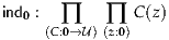
gives us a way to define a trivial dependent function out of the empty type.
The type of booleans 2 : is intended to have exactly two elements
02, 12 : 2. It is clear that we could construct this type out of coproduct
and unit types as 1 + 1. However, since it is used frequently, we give
the explicit rules here. Indeed, we are going to observe that we can
also go the other way and derive binary coproducts from Σ-types and
2.
To derive a function f : 2 → C we need c0, c1 : C and add the defining equations
| f(02) | :≡ c0, | ||
| f(12) | :≡ c1. |
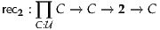
with the defining equations
| rec2(C, c0, c1, 02) | :≡ c0, | ||
| rec2(C, c0, c1, 12) | :≡ c1. |
Given C : 2 →, to derive a dependent function f : ∏(x:2) C(x) we
need c0 : C(02) and c1 : C(12), in which case we can give the defining
equations
| f(02) | :≡ c0, | ||
| f(12) | :≡ c1. |
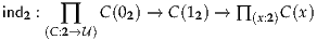
with the defining equations
| ind2(C, c0, c1, 02) | :≡ c0, | ||
| ind2(C, c0, c1, 12) | :≡ c1. |
As an example, using the induction principle we can deduce that, as we expect, every element of 2 is either 12 or 02. As before, in order to state this we use the equality types which we have not yet introduced, but we need only the fact that everything is equal to itself by reflx : x = x. Thus, we construct an element of
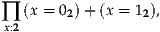 | (1.8.1) |
i.e. a function assigning to each x : 2 either an equality x = 02 or an equality x = 12. We define this element using the induction principle for 2, with C(x) :≡ (x = 02) + (x = 12); the two inputs are inl(refl02) : C(02) and inr(refl12) : C(12). In other words, our element of (1.8.1) is

We have remarked that Σ-types can be regarded as analogous to indexed
disjoint unions, while coproducts are binary disjoint unions. It is natural to
expect that a binary disjoint union A + B could be constructed as an indexed
one over the two-element type 2. For this we need a type family P : 2 →
such that P(02) ≡ A and P(12) ≡ B. Indeed, we can obtain such a family
precisely by the recursion principle for 2. (The ability to define type families by
induction and recursion, using the fact that the universe is itself a type, is a
subtle and important aspect of type theory.) Thus, we could have defined
with
| inl(a) | :≡ (02, a), | ||
| inr(b) | :≡ (12, b). |
We can apply the same idea to products and Π-types: we could have defined
Pairs could then be constructed using induction for 2:

while the projections are straightforward applications
| pr1(p) | :≡ p(02), | ||
| pr2(p) | :≡ p(12). |
We may occasionally refer to the elements 02 and 12 of 2 as “false” and “true” respectively. However, note that unlike in classical mathematics, we do not use elements of 2 as truth values or as propositions. (Instead we identify propositions with types; see §1.11.) In particular, the type A →2 is not generally the power set of A; it represents only the “decidable” subsets of A (see Chapter 3).
The rules we have introduced so far do not allow us to construct any infinite
types. The simplest infinite type we can think of (and one which is of course
also extremely useful) is the type N : of natural numbers. The elements of
N are constructed using 0 : N and the successor operation succ : N →N.
When denoting natural numbers, we adopt the usual decimal notation
1 :≡succ(0), 2 :≡succ(1), 3 :≡succ(2), ….
The essential property of the natural numbers is that we can define functions by recursion and perform proofs by induction — where now the words “recursion” and “induction” have a more familiar meaning. To construct a non-dependent function f : N → C out of the natural numbers by recursion, it is enough to provide a starting point c0 : C and a “next step” function cs : N → C → C. This gives rise to f with the defining equations
| f(0) | :≡ c0, | ||
| f(succ(n)) | :≡ cs(n, f(n)). |
As an example, we look at how to define a function on natural numbers which doubles its argument. In this case we have C :≡N. We first need to supply the value of double(0), which is easy: we put c0 :≡ 0. Next, to compute the value of double(succ(n)) for a natural number n, we first compute the value of double(n) and then perform the successor operation twice. This is captured by the recurrence cs(n, y) :≡succ(succ(y)). Note that the second argument y of cs stands for the result of the recursive call double(n).
Defining double : N →N by primitive recursion in this way, therefore, we obtain the defining equations:
| double(0) | :≡ 0 | ||
| double(succ(n)) | :≡succ(succ(double(n))). |
| double(2) | ≡double(succ(succ(0))) | ||
| ≡ cs(succ(0), double(succ(0))) | |||
| ≡succ(succ(double(succ(0)))) | |||
| ≡succ(succ(cs(0, double(0)))) | |||
| ≡succ(succ(succ(succ(double(0))))) | |||
| ≡succ(succ(succ(succ(c0)))) | |||
| ≡succ(succ(succ(succ(0)))) | |||
| ≡ 4. |
| c0 | : N →N | ||
| c0(n) | :≡ n | ||
| cs | : N → (N →N) → (N →N) | ||
| cs(m, g)(n) | :≡succ(g(n)). |
| add(0, n) | ≡ n | ||
| add(succ(m), n) | ≡succ(add(m, n)). |
As in previous cases, we can package the principle of primitive recursion into a recursor:
| recN(C, c0, cs, 0) | :≡ c0, | ||
| recN(C, c0, cs, succ(n)) | :≡ cs(n, recN(C, c0, cs, n)). |
| double | :≡recN N, 0, λn.λy.succ(succ(y)) N, 0, λn.λy.succ(succ(y)) | (1.9.1) |
| add | :≡recN N →N, λn.n, λn.λg.λm.succ(g(m)) N →N, λn.n, λn.λg.λm.succ(g(m)) . . | (1.9.2) |
We now follow the same approach as for other types, generalizing primitive
recursion to dependent functions to obtain an induction principle. Thus,
assume as given a family C : N →, an element c0 : C(0), and a function
cs : ∏(n:N) C(n) → C(succ(n)); then we can construct f : ∏(n:N) C(n) with
the defining equations:
| f(0) | :≡ c0, | ||
| f(succ(n)) | :≡ cs(n, f(n)). |

with the defining equations
| indN(C, c0, cs, 0) | :≡ c0, | ||
| indN(C, c0, cs, succ(n)) | :≡ cs(n, indN(C, c0, cs, n)). |
. From this point of view, the above induction
principle says that if we can prove P(0), and if for any n we can prove
P(succ(n)) assuming P(n), then we have P(n) for all n. This is, of
course, exactly the usual principle of proof by induction on natural
numbers.
As an example, consider how we might represent an explicit proof that + is associative. (We will not actually write out proofs in this style, but it serves as a useful example for understanding how induction is represented formally in type theory.) To derive
it is sufficient to supply
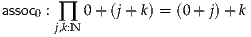
and
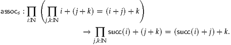
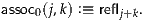
For assocs, recall that the definition of + gives succ(m) + n ≡succ(m + n), and hence
| succ(i) + (j + k) | ≡succ(i + (j + k)) and | ||
| (succ(i) + j) + k | ≡succ((i + j) + k). |

Putting these together with indN, we obtain a proof of associativity.
The natural numbers introduce an additional subtlety over the types considered up until now. In the case of coproducts, for instance, we could define a function f : A + B → C either with the recursor:
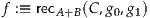
or by giving the defining equations:
| f(inl(a)) | :≡ g0(a) | ||
| f(inr(b)) | :≡ g1(b). |
| f(inl(a)) | :≡ Φ0 | ||
| f(inr(b)) | :≡ Φ1 |

In the case of the natural numbers, however, the “defining equations” of a function such as double:
| double(0) | :≡ 0 | (1.10.1) |
| double(succ(n)) | :≡succ(succ(double(n))) | (1.10.2) |
More generally, if we have a “definition” of a function f : N → C such as
| f(0) | :≡ Φ0 | ||
| f(succ(n)) | :≡ Φs |
where Φs′ is obtained from Φs by replacing all occurrences of “f(n)” by the new variable r.
This style of defining functions by recursion (or, more generally, dependent functions by induction) is so convenient that we frequently adopt it. It is called definition by pattern matching. Of course, it is very similar to how a computer programmer may define a recursive function with a body that literally contains recursive calls to itself. However, unlike the programmer, we are restricted in what sort of recursive calls we can make: in order for such a definition to be re-expressible using the recursion principle, the function f being defined can only appear in the body of f(succ(n)) as part of the composite symbol “f(n)”. Otherwise, we could write nonsense functions such as
| f(0) | :≡ 0 | ||
| f(succ(n)) | :≡ f(succ(succ(n))). |
This point will be even more important when we introduce more complicated inductive types in Chapters 5, 6 and 11. Whenever we introduce a new kind of inductive definition, we always begin by deriving its induction principle. Only then do we introduce an appropriate sort of “pattern matching” which can be justified as a shorthand for the induction principle.
As mentioned in the introduction, to show that a proposition is true in type theory corresponds to exhibiting an element of the type corresponding to that proposition. We regard the elements of this type as evidence or witnesses that the proposition is true. (They are sometimes even called proofs, but this terminology can be misleading, so we generally avoid it.) In general, however, we will not construct witnesses explicitly; instead we present the proofs in ordinary mathematical prose, in such a way that they could be translated into an element of a type. This is no different from reasoning in classical set theory, where we don’t expect to see an explicit derivation using the rules of predicate logic and the axioms of set theory.
However, the type-theoretic perspective on proofs is nevertheless different in important ways. The basic principle of the logic of type theory is that a proposition is not merely true or false, but rather can be seen as the collection of all possible witnesses of its truth. Under this conception, proofs are not just the means by which mathematics is communicated, but rather are mathematical objects in their own right, on a par with more familiar objects such as numbers, mappings, groups, and so on. Thus, since types classify the available mathematical objects and govern how they interact, propositions are nothing but special types — namely, types whose elements are proofs.
The basic observation which makes this identification feasible is that we have the following natural correspondence between logical operations on propositions, expressed in English, and type-theoretic operations on their corresponding types of witnesses.
| English | Type Theory |
| True | 1 |
| False | 0 |
| A and B | A×B |
| A or B | A + B |
| If A then B | A → B |
| A if and only if B | (A → B) × (B → A) |
| Not A | A →0 |
The point of the correspondence is that in each case, the rules for constructing and using elements of the type on the right correspond to the rules for reasoning about the proposition on the left. For instance, the basic way to prove a statement of the form “A and B” is to prove A and also prove B, while the basic way to construct an element of A×B is as a pair (a, b), where a is an element (or witness) of A and b is an element (or witness) of B. And if we want to use “A and B” to prove something else, we are free to use both A and B in doing so, analogously to how the induction principle for A×B allows us to construct a function out of it by using elements of A and of B.
Similarly, the basic way to prove an implication “if A then B” is to assume A and prove B, while the basic way to construct an element of A → B is to give an expression which denotes an element (witness) of B which may involve an unspecified variable element (witness) of type A. And the basic way to use an implication “if A then B” is deduce B if we know A, analogously to how we can apply a function f : A → B to an element of A to produce an element of B. We strongly encourage the reader to do the exercise of verifying that the rules governing the other type constructors translate sensibly into logic.
Of special note is that the empty type 0 corresponds to falsity. When speaking logically, we refer to an inhabitant of 0 as a contradiction: thus there is no way to prove a contradiction,9 while from a contradiction anything can be derived. We also define the negation of a type A as
 |
Thus, a witness of ¬A is a function A →0, which we may construct by assuming x : A and deriving an element of 0. Note that although the logic we obtain is “constructive”, as discussed in the introduction, this sort of “proof by contradiction” (assume A and derive a contradiction, concluding ¬A) is perfectly valid constructively: it is simply invoking the meaning of “negation”. The sort of “proof by contradiction” which is disallowed is to assume ¬A and derive a contradiction as a way of proving A. Constructively, such an argument would only allow us to conclude ¬¬A, and the reader can verify that there is no obvious way to get from ¬¬A (that is, from (A →0) →0) to A.
The above translation of logical connectives into type-forming operations is referred to as propositions as types: it gives us a way to translate propositions and their proofs, written in English, into types and their elements. For example, suppose we want to prove the following tautology (one of “de Morgan’s laws”):
 | (1.11.1) |
An ordinary English proof of this fact might go as follows.
Suppose not A and not B, and also suppose A or B; we will derive a contradiction. There are two cases. If A holds, then since not A, we have a contradiction. Similarly, if B holds, then since not B, we also have a contradiction. Thus we have a contradiction in either case, so not (A or B).
Now, the type corresponding to our tautology (1.11.1), according to the rules given above, is
 | (1.11.2) |
so we should be able to translate the above proof into an element of this type.
As an example of how such a translation works, let us describe how a mathematician reading the above English proof might simultaneously construct, in his or her head, an element of (1.11.2). The introductory phrase “Suppose not A and not B” translates into defining a function, with an implicit application of the recursion principle for the cartesian product in its domain (A →0) × (B →0). This introduces unnamed variables (hypotheses) of types A →0 and B →0. When translating into type theory, we have to give these variables names; let us call them x and y. At this point our partial definition of an element of (1.11.2) can be written as
with a “hole” □ of type A + B →0 indicating what remains to be done. (We could equivalently write f :≡rec(A→0)×(B→0)(A + B →0, λx.λy.□), using the recursor instead of pattern matching.) The next phrase “also suppose A or B; we will derive a contradiction” indicates filling this hole by a function definition, introducing another unnamed hypothesis z : A + B, leading to the proof state:
Now saying “there are two cases” indicates a case split, i.e. an application of the recursion principle for the coproduct A + B. If we write this using the recursor, it would be

while if we write it using pattern matching, it would be
| f((x, y))(inl(a)) | :≡□ : 0 | ||
| f((x, y))(inr(b)) | :≡□ : 0. |
| f((x, y))(inl(a)) | :≡ x(a) | ||
| f((x, y))(inr(b)) | :≡ y(b). |
As an exercise, you should verify the converse tautology “If not (Aor B), then (not A) and (not B)” by exhibiting an element of

for any types A and B, using the rules we have just introduced.
However, not all classical tautologies hold under this interpretation. For example, the rule “If not (A and B), then (not A) or (not B)” is not valid: we cannot, in general, construct an element of the corresponding type

This reflects the fact that the “natural” propositions-as-types logic of type theory is constructive. This means that it does not include certain classical principles, such as the law of excluded middle (LEM) or proof by contradiction, and others which depend on them, such as this instance of de Morgan’s law.
Philosophically, constructive logic is so-called because it confines itself to constructions that can be carried out effectively, which is to say those with a computational meaning. Without being too precise, this means there is some sort of algorithm specifying, step-by-step, how to build an object (and, as a special case, how to see that a theorem is true). This requires omission of LEM, since there is no effective procedure for deciding whether a proposition is true or false.
The constructivity of type-theoretic logic means it has an intrinsic computational meaning, which is of interest to computer scientists. It also means that type theory provides axiomatic freedom. For example, while by default there is no construction witnessing LEM, the logic is still compatible with the existence of one (see §3.4). Thus, because type theory does not deny LEM, we may consistently add it as an assumption, and work conventionally without restriction. In this respect, type theory enriches, rather than constrains, conventional mathematical practice.
We encourage the reader who is unfamiliar with constructive logic to work through some more examples as a means of getting familiar with it. See Exercises 1.12 and 1.13 for some suggestions.
So far we have discussed only propositional logic. Now we consider
predicate logic, where in addition to logical connectives like “and” and “or”
we have quantifiers “there exists” and “for all”. In this case, types
play a dual role: they serve as propositions and also as types in the
conventional sense, i.e., domains we quantify over. A predicate over a type
A is represented as a family P : A →, assigning to every element
a : A a type P(a) corresponding to the proposition that P holds for
a. We now extend the above translation with an explanation of the
quantifiers:
| English | Type Theory |
| For all x : A, P(x) holds | ∏(x:A) P(x) |
| There exists x : A such that P(x) | ∑(x:A) P(x) |
As before, we can show that tautologies of (constructive) predicate logic translate into inhabited types. For example, If for all x : A, P(x) and Q(x) then (for all x : A, P(x)) and (for all x : A, Q(x)) translates to

An informal proof of this tautology might go as follows:
Suppose for all x, P(x) and Q(x). First, we suppose given x and prove P(x). By assumption, we have P(x) and Q(x), and hence we have P(x). Second, we suppose given x and prove Q(x). Again by assumption, we have P(x) and Q(x), and hence we have Q(x).
The first sentence begins defining an implication as a function, by introducing a witness for its hypothesis:

At this point there is an implicit use of the pairing constructor to produce an element of a product type, which is somewhat signposted in this example by the words “first” and “second”:
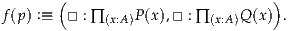
The phrase “we suppose given x and prove P(x)” now indicates defining a dependent function in the usual way, introducing a variable for its input. Since this is inside a pairing constructor, it is natural to write it as a λ-abstraction:
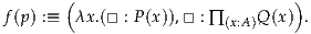
Now “we have P(x) and Q(x)” invokes the hypothesis, obtaining p(x) : P(x) ×Q(x), and “hence we have P(x)” implicitly applies the appropriate projection:
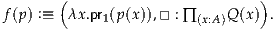
The next two sentences fill the other hole in the obvious way:
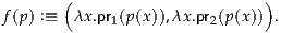
Of course, the English proofs we have been using as examples are much more verbose than those that mathematicians usually use in practice; they are more like the sort of language one uses in an “introduction to proofs” class. The practicing mathematician has learned to fill in the gaps, so in practice we can omit plenty of details, and we will generally do so. The criterion of validity for proofs, however, is always that they can be translated back into the construction of an element of the corresponding type.
As a more concrete example, consider how to define inequalities of natural numbers. One natural definition is that n ≤ m if there exists a k : N such that n + k = m. (This uses again the identity types that we will introduce in the next section, but we will not need very much about them.) Under the propositions-as-types translation, this would yield:
The reader is invited to prove the familiar properties of ≤ from this definition. For strict inequality, there are a couple of natural choices, such as
or

The former is more natural in constructive mathematics, but in this case it is actually equivalent to the latter, since N has “decidable equality” (see §3.4 and Theorem 7.2.6).
There is also another interpretation of the type ∑(x:A) P(x). Since an inhabitant of it is an element x : A together with a witness that P(x) holds, instead of regarding ∑(x:A) P(x) as the proposition “there exists an x : A such that P(x)”, we can regard it as “the type of all elements x : A such that P(x)”, i.e. as a “subtype” of A.
We will return to this interpretation in §3.5. For now, we note that it allows us to incorporate axioms into the definition of types as mathematical structures which we discussed in §1.6. For example, suppose we want to define a semigroup to be a type A equipped with a binary operation m : A → A → A (that is, a magma) and such that for all x, y, z : A we have m(x, m(y, z)) = m(m(x, y), z). This latter proposition is represented by the type
so the type of semigroups is

i.e. the subtype of Magma consisting of the semigroups. From an inhabitant of Semigroup we can extract the carrier A, the operation m, and a witness of the axiom, by applying appropriate projections. We will return to this example in §2.14.
Note also that we can use the universes in type theory to represent “higher
order logic” — that is, we can quantify over all propositions or over all
predicates. For example, we can represent the proposition for all properties
P : A →, if P(a) then P(b) as
where A : and a, b : A. However, a priori this proposition lives in a different,
higher, universe than the propositions we are quantifying over; that
is
We will return to this issue in §3.5.
We have described here a “proof-relevant” translation of propositions, where the proofs of disjunctions and existential statements carry some information. For instance, if we have an inhabitant of A + B, regarded as a witness of “A or B”, then we know whether it came from A or from B. Similarly, if we have an inhabitant of ∑(x:A) P(x), regarded as a witness of “there exists x : A such that P(x)”, then we know what the element x is (it is the first projection of the given inhabitant).
As a consequence of the proof-relevant nature of this logic, we may have “A if and only if B” (which, recall, means (A → B) × (B → A)), and yet the types A and B exhibit different behavior. For instance, it is easy to verify that “N if and only if 1”, and yet clearly N and 1 differ in important ways. The statement “N if and only if 1” tells us only that when regarded as a mere proposition, the type N represents the same proposition as 1 (in this case, the true proposition). We sometimes express “A if and only if B” by saying that A and B are logically equivalent. This is to be distinguished from the stronger notion of equivalence of types to be introduced in §2.4 and Chapter 4: although N and 1 are logically equivalent, they are not equivalent types.
In Chapter 3 we will introduce a class of types called “mere propositions” for which equivalence and logical equivalence coincide. Using these types, we will introduce a modification to the above-described logic that is sometimes appropriate, in which the additional information contained in disjunctions and existentials is discarded.
Finally, we note that the propositions-as-types correspondence can be viewed in reverse, allowing us to regard any type A as a proposition, which we prove by exhibiting an element of A. Sometimes we will state this proposition as “A is inhabited”. That is, when we say that A is inhabited, we mean that we have given a (particular) element of A, but that we are choosing not to give a name to that element. Similarly, to say that A is not inhabited is the same as to give an element of ¬A. In particular, the empty type 0 is obviously not inhabited, since ¬0 ≡ (0 →0) is inhabited by id0.10
While the previous constructions can be seen as generalizations of standard set theoretic constructions, our way of handling identity seems to be specific to type theory. According to the propositions-as-types conception, the proposition that two elements of the same type a, b : A are equal must correspond to some type. Since this proposition depends on what a and b are, these equality types or identity types must be type families dependent on two copies of A.
We may write the family as IdA : A → A →, so that IdA(a, b) is the type
representing the proposition of equality between a and b. Once we are familiar
with propositions-as-types, however, it is convenient to also use the
standard equality symbol for this; thus “a = b” will also be a notation
for the type IdA(a, b) corresponding to the proposition that a equals
b. For clarity, we may also write “a =A b” to specify the type A. If
we have an element of a =A b, we may say that a and b are equal,
or sometimes propositionally equal if we want to emphasize that
this is different from the judgmental equality a ≡ b discussed in §1.1.
Just as we remarked in §1.11 that the propositions-as-types versions of “or” and “there exists” can include more information than just the fact that the proposition is true, nothing prevents the type a = b from also including more information. Indeed, this is the cornerstone of the homotopical interpretation, where we regard witnesses of a = b as paths or equivalences between a and b in the space A. Just as there can be more than one path between two points of a space, there can be more than one witness that two objects are equal. Put differently, we may regard a = b as the type of identifications of a and b, and there may be many different ways in which a and b can be identified. We will return to the interpretation in Chapter 2; for now we focus on the basic rules for the identity type. Just like all the other types considered in this chapter, it will have rules for formation, introduction, elimination, and computation, which behave formally in exactly the same way.
The formation rule says that given a type A : and two elements a, b : A,
we can form the type (a =A b) : in the same universe. The basic way to
construct an element of a = b is to know that a and b are the same. Thus, the
introduction rule is a dependent function
called reflexivity, which says that every element of A is equal to itself (in a specified way). We regard refla as being the constant path at the point a.
In particular, this means that if a and b are judgmentally equal, a ≡ b, then we also have an element refla : a =A b. This is well-typed because a ≡ b means that also the type a =A b is judgmentally equal to a =A a, which is the type of refla.
The induction principle (i.e. the elimination rule) for the identity types is one of the most subtle parts of type theory, and crucial to the homotopy interpretation. We begin by considering an important consequence of it, the principle that “equals may be substituted for equals”, as expressed by the following:

there is a function
such that
This says that every family of types C respects equality, in the sense that applying C to equal elements of A also results in a function between the resulting types. The displayed equality states that the function associated to reflexivity is the identity function (and we shall see that, in general, the function f(x, y, p) : C(x) → C(y) is always an equivalence of types).
Indiscernability of identicals can be regarded as a recursion principle for the identity type, analogous to those given for booleans and natural numbers above. Just as recN gives a specified map N → C for any other type C of a certain sort, indiscernability of identicals gives a specified map from x =A y to certain other reflexive, binary relations on A, namely those of the form C(x) → C(y) for some unary predicate C(x). We could also formulate a more general recursion principle with respect to reflexive relations of the more general form C(x, y). However, in order to fully characterize the identity type, we must generalize this recursion principle to an induction principle, which not only considers maps out of x =A y but also families over it. Put differently, we consider not only allowing equals to be substituted for equals, but also taking into account the evidence p for the equality.
The induction principle for the identity type is called path induction, in view of the homotopical interpretation to be explained in the introduction to Chapter 2. It can be seen as stating that the family of identity types is freely generated by the elements of the form reflx : x = x.
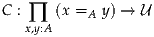
and a function
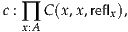
there is a function
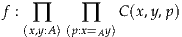
such that
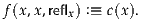
Note that just like the induction principles for products, coproducts, natural numbers, and so on, path induction allows us to define specified functions which exhibit appropriate computational behavior. Just as we have the function f : N → C defined by recursion from c0 : C and cs : N → C → C, which moreover satisfies f(0) ≡ c0 and f(succ(n)) ≡ cs(n, f(n)), we have the function f : ∏(x,y:A) ∏(p:x=Ay) C(x, y, p) defined by path induction from c : ∏(x:A) C(x, x, reflx), which moreover satisfies f(x, x, reflx) ≡ c(x).
To understand the meaning of this principle, consider first the simpler case
when C does not depend on p. Then we have C : A → A →, which we may
regard as a predicate depending on two elements of A. We are interested in
knowing when the proposition C(x, y) holds for some pair of elements
x, y : A. In this case, the hypothesis of path induction says that we know
C(x, x) holds for all x : A, i.e. that if we evaluate C at the pair x, x, we
get a true proposition — so C is a reflexive relation. The conclusion
then tells us that C(x, y) holds whenever x = y. This is exactly the
more general recursion principle for reflexive relations mentioned
above.
The general, inductive form of the rule allows C to also depend on the witness p : x = y to the identity between x and y. In the premise, we not only replace x, y by x, x, but also simultaneously replace p by reflexivity: to prove a property for all elements x, y and paths p : x = y between them, it suffices to consider all the cases where the elements are x, x and the path is reflx : x = x. If we were viewing types just as sets, it would be unclear what this buys us, but since there may be many different identifications p : x = y between x and y, it makes sense to keep track of them in considering families over the type x =A y. In Chapter 2 we will see that this is very important to the homotopy interpretation.
If we package up path induction into a single function, it takes the form:
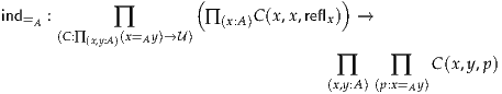
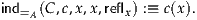
The function ind=A is traditionally called J. We leave it as an easy exercise to show that indiscernability of identicals follows from path induction.
Given a proof p : a = b, path induction requires us to replace both a and b with the same unknown element x; thus in order to define an element of a family C, for all pairs of elements of A, it suffices to define it on the diagonal. In some proofs, however, it is simpler to make use of an equation p : a = b by replacing all occurrences of b with a (or vice versa), because it is sometimes easier to do the remainder of the proof for the specific element a mentioned in the equality than for a general unknown x. This motivates a second induction principle for identity types, which says that the family of types a =A x is generated by the element refla : a = a. As we show below, this second principle is equivalent to the first; it is just sometimes a more convenient formulation.
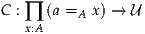
and an element

Then we obtain a function
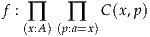
such that
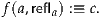
Here, C(x, p) is a family of types, where x is an element of A and p is an element of the identity type a =A x, for fixed a in A. The based path induction principle says that to define an element of this family for all x and p, it suffices to consider just the case where x is a and p is refla : a = a.
Packaged as a function, based path induction becomes:
| ind=A′ : ∏
(a:A) ∏
(C: ∏(x:A) (a=Ax)→) C(a, refla) → ∏
(x:A) ∏
(p:a=Ax) C(x, p) |

Below, we show that path induction and based path induction are equivalent. Because of this, we will sometimes be sloppy and also refer to based path induction simply as “path induction”, relying on the reader to infer which principle is meant from the form of the proof.
Remark 1.12.1. Intuitively, the induction principle for the natural numbers expresses the fact that the only natural numbers are 0 and succ(n), so if we prove a property for these cases, then we have proved it for all natural numbers. Applying this same reading to path induction, we might loosely say that path induction expresses the fact that the only path is refl, so if we prove a property for reflexivity, then we have proved it for all paths. However, this reading is quite confusing in the context of the homotopy interpretation of paths, where there may be many different ways in which two elements a and b can be identified, and therefore many different elements of the identity type! How can there be many different paths, but at the same time we have an induction principle asserting that the only path is reflexivity?
The key observation is that it is not the identity type that is inductively defined, but the identity family. In particular, path induction says that the family of types (x =A y), as x, y vary over all elements of A, is inductively defined by the elements of the form reflx. This means that to give an element of any other family C(x, y, p) dependent on a generic element (x, y, p) of the identity family, it suffices to consider the cases of the form (x, x, reflx). In the homotopy interpretation, this says that the type of triples (x, y, p), where x and y are the endpoints of the path p (in other words, the Σ-type ∑(x,y:A) (x = y)), is inductively generated by the constant loops at each point x. As we will see in Chapter 2, in homotopy theory the space corresponding to ∑(x,y:A) (x = y) is the free path space — the space of paths in A whose endpoints may vary — and it is in fact the case that any point of this space is homotopic to the constant loop at some point, since we can simply retract one of its endpoints along the given path. The analogous fact is also true in type theory: we can prove by path induction on p : x = y that (x, y, p) =∑(x,y:A) (x=y) (x, x, reflx).
Similarly, based path induction says that for a fixed a : A, the family of types (a =A y), as y varies over all elements of A, is inductively defined by the element refla. Thus, to give an element of any other family C(y, p) dependent on a generic element (y, p) of this family, it suffices to consider the case (a, refla). Homotopically, this expresses the fact that the space of paths starting at some chosen point (the based path space at that point, which type-theoretically is ∑(y:A) (a = y)) is contractible to the constant loop on the chosen point. Again, the corresponding fact is also true in type theory: we can prove by based path induction on p : a = y that (y, p) =∑(y:A) (a=y) (a, refla). Note also that according to the interpretation of Σ-types as subtypes mentioned in §1.11, the type ∑ (y:A) (a = y) can be regarded as “the type of all elements of A which are equal to a”, a type-theoretic version of the “singleton subset” {a}.
Neither path induction nor based path induction provides a way to
give an element of a family C(p) where p has two fixed endpoints a and
b. In particular, for a family C : (a =A a) → dependent on a loop,
we cannot apply path induction and consider only the case for C(refla),
and consequently, we cannot prove that all loops are reflexivity. Thus,
inductively defining the identity family does not prohibit non-reflexivity
paths in specific instances of the identity type. In other words, a path
p : x = x may be not equal to reflexivity as an element of (x = x), but
the pair (x, p) will nevertheless be equal to the pair (x, reflx) as elements
of ∑(y:A) (x = y).
The two induction principles for the identity type introduced above are equivalent. It is easy to see that path induction follows from the based path induction principle. Indeed, let us assume the premises of path induction:
| C | : ∏
x,y:A (x =A y) →, | ||
| c | : ∏ x:AC(x, x, reflx). |
| C′ | : ∏
y:A (x =A y) →, | ||
| C′ | :≡ C(x), | ||
| c′ | : C′(x, reflx), | ||
| c′ | :≡ c(x). |
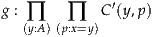 |
with the defining equality
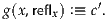 " class="math-display" >
Now we observe that g’s codomain is equal to C(x, y, p). Thus, discharging our assumption x : A, we can derive a function
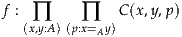
with the required judgmental equality f(x, x, reflx) ≡ g(x, reflx) :≡ c′:≡ c(x).
Another proof of this fact is to observe that any such f can be obtained as an instance of ind=A′ so it suffices to define ind=A in terms of ind=A′ as

The other direction is a bit trickier; it is not clear how we can use a particular instance of path induction to derive a particular instance of based path induction. What we can do instead is to construct one instance of path induction which shows all possible instantiations of based path induction at once. Define
| D | : ∏
x,y:A (x =A y) →, | ||
| D(x, y, p) | :≡ ∏
C:∏(z:A)(x=Az)→C(x, reflx) → C(y, p). |
| d | : ∏ x:AD(x, x, reflx), | ||
| d | :≡ λx.λC.λ(c:C(x, reflx)).c |
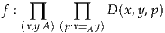
with f(x, x, reflx) :≡ d(x). Unfolding the definition of D, we can expand the type of f:
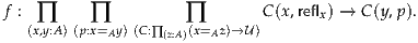
Now given x : A and p : a =A x, we can derive the conclusion of based path induction:
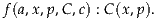
Notice that we also obtain the correct definitional equality.
Another proof is to observe that any use of based path induction is an instance of ind=A′ and to define
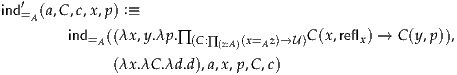
Note that the construction given above uses universes. That is, if we want
to model ind=A′ with C : ∏(x:A) (a =A x) →i, we need to use ind=A
with
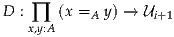
since D quantifies over all C of the given type. While this is compatible with our definition of universes, it is also possible to derive ind=A′ without using universes: we can show that ind=A entails Lemmas 2.3.1 and 3.11.8, and that these two principles imply ind=A′ directly. We leave the details to the reader as Exercise 1.7.
We can use either of the foregoing formulations of identity types to establish that equality is an equivalence relation, that every function preserves equality and that every family respects equality. We leave the details to the next chapter, where this will be derived and explained in the context of homotopy type theory.
Remark 1.12.2. We emphasize that despite having some unfamiliar features, propositional equality is the equality of mathematics in homotopy type theory. This distinction does not belong to judgmental equality, which is rather a metatheoretic feature of the rules of type theory. For instance, the associativity of addition for natural numbers proven in §1.9 is a propositional equality, not a judgmental one. The same is true of the commutative law (Exercise 1.16). Even the very simple commutativity n + 1 = 1 + n is not a judgmental equality for a generic n (though it is judgmental for any specific n, e.g. 3 + 1 ≡ 1 + 3, since both are judgmentally equal to 4 by the computation rules defining +). We can only prove such facts by using the identity type, since we can only apply the induction principle for N with a type as output (not a judgment).
Finally, let us also say something about disequality, which is negation of equality:11
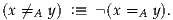 |
If x≠y, we say that x and y are unequal or not equal. Just like negation, disequality plays a less important role here than it does in classical mathematics. For example, we cannot prove that two things are equal by proving that they are not unequal: that would be an application of the classical law of double negation, see §3.4.
Sometimes it is useful to phrase disequality in a positive way. For example, in Theorem 11.2.4 we shall prove that a real number x has an inverse if, and only if, its distance from 0 is positive, which is a stronger requirement than x≠0.
The type theory presented here is a version of Martin-Löf’s intuitionistic type theory [ML98, ML75, ML82, ML84], which itself is based on and influenced by the foundational work of Brouwer [Bee85], Heyting [Hey66], Scott [Sco70], de Bruijn [dB73], Howard [How80], Tait [Tai67, Tai68], and Lawvere [Law06]. Three principal variants of Martin-Löf’s type theory underlie the NuPRL [CAB+86], Coq [Coq12], and Agda [Nor07] computer implementations of type theory. The theory given here differs from these formulations in a number of respects, some of which are critical to the homotopy interpretation, while others are technical conveniences or involve concepts that have not yet been studied in the homotopical setting.
Most significantly, the type theory described here is derived from the intensional version of Martin-Löf’s type theory [ML75], rather than the extensional version [ML82]. Whereas the extensional theory makes no distinction between judgmental and propositional equality, the intensional theory regards judgmental equality as purely definitional, and admits a much broader, proof-relevant interpretation of the identity type that is central to the homotopy interpretation. From the homotopical perspective, extensional type theory confines itself to homotopically discrete sets (see §3.1), whereas the intensional theory admits types with higher-dimensional structure. The NuPRL system [CAB+86] is extensional, whereas both Coq [Coq12] and Agda [Nor07] are intensional. Among intensional type theories, there are a number of variants that differ in the structure of identity proofs. The most liberal interpretation, on which we rely here, admits a proof-relevant interpretation of equality, whereas more restricted variants impose restrictions such as uniqueness of identity proofs (UIP) [Str93], stating that any two proofs of equality are judgmentally equal, and Axiom K [Str93], stating that the only proof of equality is reflexivity (up to judgmental equality). These additional requirements may be selectively imposed in the Coq and Agda systems.
Another point of variation among intensional theories is the strength of judgmental equality, particularly as regards objects of function type. Here we include the uniqueness principle (η-conversion) f ≡ λx.f(x), as a principle of judgmental equality. This principle is used, for example, in §4.9, to show that univalence implies propositional function extensionality. Uniqueness principles are sometimes considered for other types. For instance, the uniqueness principle for cartesian products would be a judgmental version of the propositional equality uppt which we constructed in §1.5, saying that u ≡ (pr1(u), pr2(u)). This and the corresponding version for dependent pairs would be reasonable choices (which we did not make), but we cannot include all such rules, because the corresponding uniqueness principle for identity types would trivialize all the higher homotopical structure. So we are forced to leave it out, and the question then becomes where to draw the line. With regards to inductive types, we discuss these points further in §5.5.
It is important for our purposes that (propositional) equality of functions is taken to be extensional (in a different sense than that used above!). This is not a consequence of the rules in this chapter; it will be expressed by Axiom 2.9.3. This decision is significant for our purposes, because it specifies that equality of functions is as expected in mathematics. Although we include Axiom 2.9.3 as an axiom, it may be derived from the univalence axiom and the uniqueness principle for functions (see §4.9), as well as from the existence of an interval type (see Lemma 6.3.2).
Regarding inductive types such as products, Σ-types, coproducts, natural numbers, and so on (see Chapter 5), there are additional choices regarding precisely how to formulate induction and recursion. Formally, one may describe type theory by taking either pattern matching or induction principles as basic and deriving the other; see Appendix A. However, pattern matching in general is not yet well understood from the homotopical perspective (in particular, “nested” or “deep” pattern matching is difficult to make general sense of for higher inductive types). Moreover, it can be dangerous unless sufficient care is taken: for instance, the form of pattern matching implemented by default in Agda allows proving Axiom K. For these reasons, we have chosen to regard the induction principle as the basic property of an inductive definition, with pattern matching justified in terms of induction.
Unlike the type theory of Coq, we do not include a primitive type of propositions. Instead, as discussed in §1.11, we embrace the propositions-as-types (PAT) principle, identifying propositions with types. This was suggested originally by de Bruijn [dB73], Howard [How80], Tait [Tai68], and Martin-Löf [ML98]. (Our decision is explained more fully in §§3.2 and 3.3.)
We do, however, include a full cumulative hierarchy of universes, so that
the type formation and equality judgments become instances of the
membership and equality judgments for a universe. As a convenience, we
regard objects of a universe as types, rather than as codes for types; in the
terminology of [ML84], this means we use “Russell-style universes” rather
than “Tarski-style universes”. An alternative would be to use Tarski-style
universes, with an explicit coercion function required to make an element
A : of a universe into a type El(A), and just say that the coercion is omitted
when working informally.
We also treat the universe hierarchy as cumulative, in that every type in i
is also in j for each j ≥ i. There are different ways to implement cumulativity
formally: the simplest is just to include a rule that if A : i then A : j.
However, this has the annoying consequence that for a type family
B : A →i we cannot conclude B : A →j, although we can conclude
λa.B(a) : A →j. A more sophisticated approach that solves this problem is
to introduce a judgmental subtyping relation <: generated by i <: j, but
this makes the type theory more complicated to study. Another alternative
would be to include an explicit coercion function ↑: i →j, which could be
omitted when working informally.
It is also not necessary that the universes be indexed by natural numbers
and linearly ordered. For some purposes, it is more appropriate to assume
only that every universe is an element of some larger universe, together with
a “directedness” property that any two universes are jointly contained in
some larger one. There are many other possible variations, such as including a
universe “ω” that contains all i (or even higher “large cardinal” type
universes), or by internalizing the hierarchy into a type family λi.i. The
latter is in fact done in Agda.
The path induction principle for identity types was formulated by Martin-Löf [ML98]. The based path induction rule in the setting of Martin-Löf type theory is due to Paulin-Mohring [PM93]; it can be seen as an intensional generalization of the concept of “pointwise functionality” for hypothetical judgments from NuPRL [CAB+86, Section 8.1]. The fact that Martin-Löf’s rule implies Paulin-Mohring’s was proved by Streicher using Axiom K (see §7.2), by Altenkirch and Goguen as in §1.12, and finally by Hofmann without universes (as in Exercise 1.7); see [Str93, §1.3 and Addendum].
Exercise 1.1. Given functions f : A → B and g : B → C, define their composite g∘f : A → C. Show that we have h∘ (g∘f) ≡ (h∘g) ∘f.
Exercise 1.2. Derive the recursion principle for products recA×B using only the projections, and verify that the definitional equalities are valid. Do the same for Σ-types.
Exercise 1.3. Derive the induction principle for products indA×B, using only the projections and the propositional uniqueness principle uppt. Verify that the definitional equalities are valid. Generalize uppt to Σ-types, and do the same for Σ-types. (This requires concepts from Chapter 2.)
Exercise 1.4. Assuming as given only the iterator for natural numbers
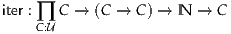
with the defining equations
| iter(C, c0, cs, 0) | :≡ c0, | ||
| iter(C, c0, cs, succ(n)) | :≡ cs(iter(C, c0, cs, n)), |
Exercise 1.5. Show that if we define A+B :≡ ∑(x:2) rec2(, A, B, x), then
we can give a definition of indA+B for which the definitional equalities
stated in §1.7 hold.
Exercise 1.6. Show that if we define A×B :≡ ∏(x:2) rec2(, A, B, x),
then we can give a definition of indA×B for which the definitional
equalities stated in §1.5 hold propositionally (i.e. using equality types).
(This requires the function extensionality axiom, which is introduced in §2.9.)
Exercise 1.7. Give an alternative derivation of ind=A′ from ind=A which avoids the use of universes. (This is easiest using concepts from later chapters.)
Exercise 1.8. Define multiplication and exponentiation using recN. Verify that (N, +, 0, ×, 1) is a semiring using only indN. You will probably also need to use symmetry and transitivity of equality, Lemmas 2.1.1 and 2.1.2.
Exercise 1.9. Define the type family Fin : N → mentioned at the end
of §1.3, and the dependent function fmax : ∏(n:N) Fin(n + 1) mentioned
in §1.4.
Exercise 1.10. Show that the Ackermann function ack : N →N →N is definable using only recN satisfying the following equations:
| ack(0, n) | ≡succ(n), | ||
| ack(succ(m), 0) | ≡ack(m, 1), | ||
| ack(succ(m), succ(n)) | ≡ack(m, ack(succ(m), n)). |
Exercise 1.12. Using the propositions as types interpretation, derive the following tautologies.
Exercise 1.13. Using propositions-as-types, derive the double negation of the principle of excluded middle, i.e. prove not (not (P or not P)).
Exercise 1.14. Why do the induction principles for identity types not allow us to construct a function f : ∏(x:A) ∏(p:x=x) (p = reflx) with the defining equation
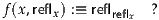
The central new idea in homotopy type theory is that types can be regarded as spaces in homotopy theory, or higher-dimensional groupoids in category theory.
We begin with a brief summary of the connection between homotopy theory and higher-dimensional category theory. In classical homotopy theory, a space X is a set of points equipped with a topology, and a path between points x and y is represented by a continuous map p : [0, 1] → X, where p(0) = x and p(1) = y. This function can be thought of as giving a point in X at each “moment in time”. For many purposes, strict equality of paths (meaning, pointwise equal functions) is too fine a notion. For example, one can define operations of path concatenation (if p is a path from x to y and q is a path from y to z, then the concatenation p▪q is a path from x to z) and inverses (p-1 is a path from y to x). However, there are natural equations between these operations that do not hold for strict equality: for example, the path p▪p-1 (which walks from x to y, and then back along the same route, as time goes from 0 to 1) is not strictly equal to the identity path (which stays still at x at all times).
The remedy is to consider a coarser notion of equality of paths called homotopy. A homotopy between a pair of continuous maps f : X1 → X2 and g : X1 → X2 is a continuous map H : X1 × [0, 1] → X2 satisfying H(x, 0) = f(x) and H(x, 1) = g(x). In the specific case of paths p and q from x to y, a homotopy is a continuous map H : [0, 1] × [0, 1] → X such that H(s, 0) = p(s) and H(s, 1) = q(s) for all s ∈ [0, 1]. In this case we require also that H(0, t) = x and H(1, t) = y for all t ∈ [0, 1], so that for each t the function H(–, t) is again a path from x to y; a homotopy of this sort is said to be endpoint-preserving or rel endpoints. Such a homotopy is the image in X of a square that fills in the space between p and q, which can be thought of as a “continuous deformation” between p and q, or a 2-dimensional path between paths.
For example, because p▪p-1 walks out and back along the same route, you know that you can continuously shrink p▪p-1 down to the identity path—it won’t, for example, get snagged around a hole in the space. Homotopy is an equivalence relation, and operations such as concatenation, inverses, etc., respect it. Moreover, the homotopy equivalence classes of loops at some point x0 (where two loops p and q are equated when there is a based homotopy between them, which is a homotopy H as above that additionally satisfies H(0, t) = H(1, t) = x0 for all t) form a group called the fundamental group. This group is an algebraic invariant of a space, which can be used to investigate whether two spaces are homotopy equivalent (there are continuous maps back and forth whose composites are homotopic to the identity), because equivalent spaces have isomorphic fundamental groups.
Because homotopies are themselves a kind of 2-dimensional path, there is a natural notion of 3-dimensional homotopy between homotopies, and then homotopy between homotopies between homotopies, and so on. This infinite tower of points, path, homotopies, homotopies between homotopies, …, equipped with algebraic operations such as the fundamental group, is an instance of an algebraic structure called a (weak) ∞-groupoid. An ∞-groupoid consists of a collection of objects, and then a collection of morphisms between objects, and then morphisms between morphisms, and so on, equipped with some complex algebraic structure; a morphism at level k is called a k-morphism. Morphisms at each level have identity, composition, and inverse operations, which are weak in the sense that they satisfy the groupoid laws (associativity of composition, identity is a unit for composition, inverses cancel) only up to morphisms at the next level, and this weakness gives rise to further structure. For example, because associativity of composition of morphisms p▪ (q▪r) = (p▪q) ▪r is itself a higher-dimensional morphism, one needs an additional operation relating various proofs of associativity: the various ways to reassociate p▪ (q▪ (r▪s)) into ((p▪q) ▪r) ▪s give rise to Mac Lane’s pentagon. Weakness also creates non-trivial interactions between levels.
Every topological space X has a fundamental ∞-groupoid whose k-morphisms are the k-dimensional paths in X. The weakness of the ∞-groupoid corresponds directly to the fact that paths form a group only up to homotopy, with the (k + 1)-paths serving as the homotopies between the k-paths. Moreover, the view of a space as an ∞-groupoid preserves enough aspects of the space to do homotopy theory: the fundamental ∞-groupoid construction is adjoint to the geometric realization of an ∞-groupoid as a space, and this adjunction preserves homotopy theory (this is called the homotopy hypothesis/theorem, because whether it is a hypothesis or theorem depends on how you define ∞-groupoid). For example, you can easily define the fundamental group of an ∞-groupoid, and if you calculate the fundamental group of the fundamental ∞-groupoid of a space, it will agree with the classical definition of fundamental group of that space. Because of this correspondence, homotopy theory and higher-dimensional category theory are intimately related.
Now, in homotopy type theory each type can be seen to have the structure of an ∞-groupoid. Recall that for any type A, and any x, y : A, we have an identity type x =A y, also written IdA(x, y) or just x = y. Logically, we may think of elements of x = y as evidence that x and y are equal, or as identifications of x with y. Furthermore, type theory (unlike, say, first-order logic) allows us to consider such elements of x =A y also as individuals which may be the subjects of further propositions. Therefore, we can iterate the identity type: we can form the type p =(x=Ay) q of identifications between identifications p, q, and the type r =(p=(x= Ay)q) s, and so on. The structure of this tower of identity types corresponds precisely to that of the continuous paths and (higher) homotopies between them in a space, or an ∞-groupoid.
Thus, we will frequently refer to an element p : x =A y as a path from x to y; we call x its start point and y its end point. Two paths p, q : x =A y with the same start and end point are said to be parallel, in which case an element r : p =(x=Ay) q can be thought of as a homotopy, or a morphism between morphisms; we will often refer to it as a 2-path or a 2-dimensional path Similarly, r =(p=(x= Ay)q) s is the type of 3-dimensional paths between two parallel 2-dimensional paths, and so on. If the type A is “set-like”, such as N, these iterated identity types will be uninteresting (see §3.1), but in the general case they can model non-trivial homotopy types.
An important difference between homotopy type theory and classical homotopy theory is that homotopy type theory provides a synthetic description of spaces, in the following sense. Synthetic geometry is geometry in the style of Euclid [EucBC]: one starts from some basic notions (points and lines), constructions (a line connecting any two points), and axioms (all right angles are equal), and deduces consequences logically. This is in contrast with analytic geometry, where notions such as points and lines are represented concretely using cartesian coordinates in Rn—lines are sets of points—and the basic constructions and axioms are derived from this representation. While classical homotopy theory is analytic (spaces and paths are made of points), homotopy type theory is synthetic: points, paths, and paths between paths are basic, indivisible, primitive notions.
Moreover, one of the amazing things about homotopy type theory is that all of the basic constructions and axioms—all of the higher groupoid structure—-arises automatically from the induction principle for identity types. Recall from §1.12 that this says that if
then
In other words, given dependent functions
| D | : ∏
x,y:A (x = y) → | ||
| d | : ∏ a:A D(a, a, refla) |
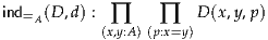
such that
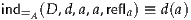 | (2.0.1) |
for every a : A. Usually, every time we apply this induction rule we will either not care about the specific function being defined, or we will immediately give it a different name.
Informally, the induction principle for identity types says that if we want to construct an object (or prove a statement) which depends on an inhabitant p : x =A y of an identity type, then it suffices to perform the construction (or the proof) in the special case when x and y are the same (judgmentally) and p is the reflexivity element reflx : x = x (judgmentally). When writing informally, we may express this with a phrase such as “by induction, it suffices to assume…”. This reduction to the “reflexivity case” is analogous to the reduction to the “base case” and “inductive step” in an ordinary proof by induction on the natural numbers, and also to the “left case” and “right case” in a proof by case analysis on a disjoint union or disjunction.
The “conversion rule” (2.0.1) is less familiar in the context of proof by induction on natural numbers, but there is an analogous notion in the related concept of definition by recursion. If a sequence (an)n∈N is defined by giving a0 and specifying an+1 in terms of an, then in fact the 0th term of the resulting sequence is the given one, and the given recurrence relation relating an+1 to an holds for the resulting sequence. (This may seem so obvious as to not be worth saying, but if we view a definition by recursion as an algorithm for calculating values of a sequence, then it is precisely the process of executing that algorithm.) The rule (2.0.1) is analogous: it says that if we define an object f(p) for all p : x = y by specifying what the value should be when p is reflx : x = x, then the value we specified is in fact the value of f(reflx).
This induction principle endows each type with the structure of an ∞-groupoid, and each function between two types the structure of an ∞-functor between two such groupoids. This is interesting from a mathematical point of view, because it gives a new way to work with ∞-groupoids. It is interesting from a type-theoretic point of view, because it reveals new operations that are associated with each type and function. In the remainder of this chapter, we begin to explore this structure.
We now derive from the induction principle the beginnings of the structure of a higher groupoid. We begin with symmetry of equality, which, in topological language, means that “paths can be reversed”.
Lemma 2.1.1. For every type Aand every x, y : Athere is a function
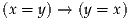 |
denoted p p-1, such that reflx-1 ≡reflx for each x : A. We call p-1 the inverse of
p.
p-1, such that reflx-1 ≡reflx for each x : A. We call p-1 the inverse of
p.
Since this is our first time stating something as a “Lemma” or “Theorem”, let us pause to consider what that means. Recall that propositions (statements susceptible to proof) are identified with types, whereas lemmas and theorems (statements that have been proven) are identified with inhabited types. Thus, the statement of a lemma or theorem should be translated into a type, as in §1.11, and its proof translated into an inhabitant of that type. According to the interpretation of the universal quantifier “for every”, the type corresponding to Lemma 2.1.1 is
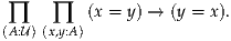
The proof of Lemma 2.1.1 will consist of constructing an element of this type,
i.e. deriving the judgment f : ∏(A:) ∏(x,y:A) (x = y) → (y = x) for some f.
We then introduce the notation (–)-1 for this element f, in which the
arguments A, x, and y are omitted and inferred from context. (As remarked in
§1.1, the secondary statement “reflx-1 ≡reflx for each x : A” should be
regarded as a separate judgment.)
First proof. Assume given A : , and let D : ∏(x,y:A) (x = y) → be the type
family defined by D(x, y, p) :≡ (y = x). In other words, D is a function
assigning to any x, y : A and p : x = y a type, namely the type y = x. Then we
have an element
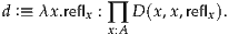 |
Thus, the induction principle for identity types gives us an element
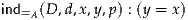 |
for each p : (x = y). We can now define the desired function (–)-1 to be λp.ind=A(D, d, x, y, p), i.e. we set p-1 :≡ind=A(D, d, x, y, p). The conversion rule (2.0.1) gives reflx-1 ≡reflx, as required. __
We have written out this proof in a very formal style, which may be helpful while the induction rule on identity types is unfamiliar. To be even more formal, we could say that Lemma 2.1.1 and its proof together consist of the judgment
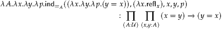
Second proof. We want to construct, for each x, y : A and p : x = y, an element p-1 : y = x. By induction, it suffices to do this in the case when y is x and p is reflx. But in this case, the type x = y of p and the type y = x in which we are trying to construct p-1 are both simply x = x. Thus, in the “reflexivity case”, we can define reflx-1 to be simply reflx. The general case then follows by the induction principle, and the conversion rule reflx-1 ≡ reflx is precisely the proof in the reflexivity case that we gave. __
We will write out the next few proofs in both styles, to help the reader become accustomed to the latter one. Next we prove the transitivity of equality, or equivalently we “concatenate paths”.
Lemma 2.1.2. For every type Aand every x, y, z : Athere is a function
 |
written p q
q p▪q, such that reflx ▪reflx ≡reflx for any x : A. We call p▪qthe
concatenation or composite of pand q.
p▪q, such that reflx ▪reflx ≡reflx for any x : A. We call p▪qthe
concatenation or composite of pand q.
First proof. Let D : ∏(x,y:A) (x = y) → be the type family
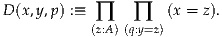 |
Note that D(x, x, reflx) ≡ ∏(z:A) ∏(q:x=z) (x = z). Thus, in order to apply the induction principle for identity types to this D, we need a function of type
 | (2.1.3) |
which is to say, of type
Now let E : ∏(x,z:A) ∏(q:x=z) be the type family E(x, z, q) :≡ (x = z). Note
that E(x, x, reflx) ≡ (x = x). Thus, we have the function
 |
By the induction principle for identity types applied to E, we obtain a function
 |
But E(x, z, q) ≡ (x = z), so the type of d is (2.1.3). Thus, we can use this function d and apply the induction principle for identity types to D, to obtain our desired function of type
 |
The conversion rules for the two induction principles give us reflx ▪reflx ≡reflx for any x : A. __
Second proof. We want to construct, for every x, y, z : A and every p : x = y and q : y = z, an element of x = z. By induction on p, it suffices to assume that y is x and p is reflx. In this case, the type y = z of q is x = z. Now by induction on q, it suffices to assume also that z is x and q is reflx. But in this case, x = z is x = x, and we have reflx : (x = x). __
The reader may well feel that we have given an overly convoluted proof of this lemma. In fact, we could stop after the induction on p, since at that point what we want to produce is an equality x = z, and we already have such an equality, namely q. Why do we go on to do another induction on q?
The answer is that, as described in the introduction, we are doing proof-relevant mathematics. When we prove a lemma, we are defining an inhabitant of some type, and it can matter what specific element we defined in the course of the proof, not merely the type inhabited by that element (that is, the statement of the lemma). Lemma 2.1.2 has three obvious proofs: we could do induction over p, induction over q, or induction over both of them. If we proved it three different ways, we would have three different elements of the same type. It’s not hard to show that these three elements are equal (see Exercise 2.1), but as they are not definitionally equal, there can still be reasons to prefer one over another.
In the case of Lemma 2.1.2, the difference hinges on the computation rule. If we proved the lemma using a single induction over p, then we would end up with a computation rule of the form refly ▪q ≡ q. If we proved it with a single induction over q, we would have instead p▪refly ≡ p, while proving it with a double induction (as we did) gives only reflx ▪reflx ≡reflx.
The asymmetrical computation rules can sometimes be convenient when doing formalized mathematics, as they allow the computer to simplify more things automatically. However, in informal mathematics, and arguably even in the formalized case, it can be confusing to have a concatenation operation which behaves asymmetrically and to have to remember which side is the “special” one. Treating both sides symmetrically makes for more robust proofs; this is why we have given the proof that we did. (However, this is admittedly a stylistic choice.)
The table below summarizes the “equality”, “homotopical”, and “higher-groupoid” points of view on what we have done so far.
In practice, transitivity is often applied to prove an equality by a chain of intermediate steps. We will use the common notation for this such as a = b = c = d. If the intermediate expressions are long, or we want to specify the witness of each equality, we may write
| a | = b | (by p) | ||||
| = c | (by q) | |||||
| = d | (by r). |
| a | = b | (by p) | ||||
| ≡ c | ||||||
| = d | (by r) |
Now, because of proof-relevance, we can’t stop after proving “symmetry” and “transitivity” of equality: we need to know that these operations on equalities are well-behaved. (This issue is invisible in set theory, where symmetry and transitivity are mere properties of equality, rather than structure on paths.) From the homotopy-theoretic point of view, concatenation and inversion are just the “first level” of higher groupoid structure — we also need coherence laws on these operations, and analogous operations at higher dimensions. For instance, we need to know that concatenation is associative, and that inversion provides inverses with respect to concatenation.
Lemma 2.1.4. Suppose A : , that x, y, z, w : Aand that p : x = yand q : y = z
and r : z = w. We have the following:
Note, in particular, that (i)–(iv) are themselves propositional equalities, living in the identity types of identity types, such as p = x=yq for p, q : x = y. Topologically, they are paths of paths, i.e. homotopies. It is a familiar fact in topology that when we concatenate a path p with the reversed path p-1, we don’t literally obtain a constant path (which corresponds to the equality refl in type theory) — instead we have a homotopy, or higher path, from p▪p-1 to the constant path.
Proof of Lemma 2.1.4. All the proofs use the induction principle for equalities.
be the type family given
by
 |
Then D(x, x, reflx) is reflx = reflx ▪reflx. Since reflx ▪reflx ≡reflx, it follows that D(x, x, reflx) ≡ (reflx = reflx). Thus, there is a function
 |
Now the induction principle for identity types gives an element ind=A(D, d, p) : (p = p▪refly) for each p : x = y. The other equality is proven similarly.
Second proof: by induction on p, it suffices to assume that y is x and that p is reflx. But in this case, we have reflx ▪reflx ≡reflx.
be the type family given
by
 |
Then D(x, x, reflx) is reflx-1 ▪reflx = reflx. Since reflx-1 ≡reflx and reflx ▪reflx ≡reflx, we get that D(x, x, reflx) ≡ (reflx = reflx). Hence we find the function
 |
Now path induction gives an element ind=A(D, d, p) : p-1 ▪p = refly for each p : x = y in A. The other equality is similar.
Second proof By induction, it suffices to assume p is reflx. But in this case, we have p-1 ▪p ≡reflx-1 ▪reflx ≡reflx.
be the type family given
by
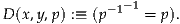 |
Then D(x, x, reflx) is the type (reflx-1-1 = reflx). But since reflx-1 ≡reflx for each x : A, we have reflx-1-1 ≡reflx-1 ≡reflx, and thus D(x, x, reflx) ≡ (reflx = reflx). Hence we find the function
 |
Now path induction gives an element ind=A(D, d, p) : p-1-1 = p for each p : x = y.
Second proof: by induction, it suffices to assume p is reflx. But in this case, we have p-1-1 ≡refl x-1-1 ≡reflx.
be the type family given
by
 |
Then D1(x, x, reflx) is
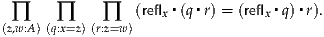 |
To construct an element of this type, let D2 : ∏(x,z:A) ∏(q:x=z) be the
type family
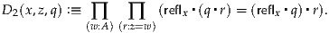 |
Then D2(x, x, reflx) is
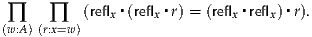 |
To construct an element of this type, let D3 : ∏(x,w:A) ∏(r:x=w) be the
type family
 |
Then D3(x, x, reflx) is
 |
which is definitionally equal to the type (reflx = reflx), and is therefore inhabited by reflreflx. Applying the path induction rule three times, therefore, we obtain an element of the overall desired type.
Second proof: by induction, it suffices to assume p, q, and r are all reflx. But in this case, we have
| p▪ (q▪r) | ≡reflx ▪ (reflx ▪reflx) | ||
| ≡reflx | |||
| ≡ (reflx ▪reflx) ▪reflx | |||
| ≡ (p▪q) ▪r. |
Remark 2.1.5. There are other ways to define these higher paths. For instance, in Lemma 2.1.4(iv) we might do induction only over one or two paths rather than all three. Each possibility will produce a definitionally different proof, but they will all be equal to each other. Such an equality between any two particular proofs can, again, be proven by induction, reducing all the paths in question to reflexivities and then observing that both proofs reduce themselves to reflexivities.
In view of Lemma 2.1.4(iv), we will often write p▪q▪r for (p▪q) ▪r, and similarly p▪q▪r▪s for ((p▪q) ▪r) ▪s and so on. We choose left-associativity for definiteness, but it makes no real difference. We generally trust the reader to insert instances of Lemma 2.1.4(iv) to reassociate such expressions as necessary.
We are still not really done with the higher groupoid structure: the paths (i)–(iv) must also satisfy their own higher coherence laws, which are themselves higher paths, and so on “all the way up to infinity” (this can be made precise using e.g. the notion of a globular operad). However, for most purposes it is unnecessary to make the whole infinite-dimensional structure explicit. One of the nice things about homotopy type theory is that all of this structure can be proven starting from only the inductive property of identity types, so we can make explicit as much or as little of it as we need.
In particular, in this book we will not need any of the complicated combinatorics involved in making precise notions such as “coherent structure at all higher levels”. In addition to ordinary paths, we will use paths of paths (i.e. elements of a type p = x=Ayq), which as remarked previously we call 2-paths or 2-dimensional paths, and perhaps occasionally paths of paths of paths (i.e. elements of a type r = p=x=Ayqs), which we call 3-paths or 3-dimensional paths. It is possible to define a general notion of n-dimensional path (see Exercise 2.4), but we will not need it.
We will, however, use one particularly important and simple case of higher paths, which is when the start and end points are the same. In set theory, the proposition a = a is entirely uninteresting, but in homotopy theory, paths from a point to itself are called loops and carry lots of interesting higher structure. Thus, given a type A with a point a : A, we define its loop space Ω(A, a) to be the type a =A a. We may sometimes write simply ΩA if the point a is understood from context.
Since any two elements of ΩA are paths with the same start and end points, they can be concatenated; thus we have an operation ΩA× ΩA → ΩA. More generally, the higher groupoid structure of A gives ΩA the analogous structure of a “higher group”.
It can also be useful to consider the loop space of the loop space of A, which is the space of 2-dimensional loops on the identity loop at a. This is written Ω2(A, a) and represented in type theory by the type refla =(a=Aa) refla. While Ω2(A, a), as a loop space, is again a “higher group”, it now also has some additional structure resulting from the fact that its elements are 2-dimensional loops between 1-dimensional loops.
Proof. First, observe that the composition of 1-loops ΩA× ΩA → ΩA induces an operation
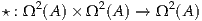
as follows: consider elements a, b, c : A and 1- and 2-paths,
| p | : a = b, | r | : b = c | ||||
| q | : a = b, | s | : b = c | ||||
| α | : p = q, | β | : r = s |
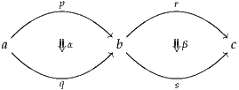
Composing the upper and lower 1-paths, respectively, we get two paths p▪r, q▪s : a = c, and there is then a “horizontal composition”
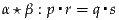 |
between them, defined as follows. First, we define α ▪r r : p▪r = q▪r by path induction on r, so that
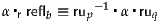
where rup : p = p▪reflb is the right unit law from Lemma 2.1.4(i). We could similarly define ▪r by induction on α, or on all paths in sight, resulting in different judgmental equalities, but for present purposes the definition by induction on r will make things simpler. Similarly, we define q ▪l β : q▪r = q▪s by induction on q, so that
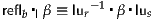
where lur denotes the left unit law. The operations ▪l and ▪r are called whiskering. Next, since α ▪r r and q ▪l β are composable 2-paths, we can define the horizontal composition by:
Now suppose that a ≡ b ≡ c, so that all the 1-paths p, q, r, and s are elements of Ω(A, a), and assume moreover that p ≡ q ≡ r ≡ s ≡refla, so that α : refla = refla and β : refla = refla are composable in both orders. In that case, we have
| α⋆β | ≡ (α ▪r refla) ▪ (refla ▪l β) | ||
| = rurefla-1 ▪α▪ru refla ▪lurefla-1 ▪β▪lu refla | |||
| ≡reflrefla-1 ▪α▪refl refla ▪reflrefla-1 ▪β▪refl refla | |||
| = α▪β. |
and we similarly learn that

But, in general, the two ways of defining horizontal composition agree, α⋆β = α⋆′β, as we can see by induction on α and β and then on the two remaining 1-paths, to reduce everything to reflexivity. Thus we have

The foregoing fact, which is known as the Eckmann–Hilton argument, comes from classical homotopy theory, and indeed it is used in Chapter 8 below to show that the higher homotopy groups of a type are always abelian groups. The whiskering and horizontal composition operations defined in the proof are also a general part of the ∞-groupoid structure of types. They satisfy their own laws (up to higher homotopy), such as
and so on. From now on, we trust the reader to apply path induction whenever needed to define further operations of this sort and verify their properties.
As this example suggests, the algebra of higher path types is much more intricate than just the groupoid-like structure at each level; the levels interact to give many further operations and laws, as in the study of iterated loop spaces in homotopy theory. Indeed, as in classical homotopy theory, we can make the following general definitions:
Definition 2.1.7. A pointed type (A, a) is a type A : together with a
point a : A, called its basepoint. We write ∙ :≡ ∑(A:) A for the type of
pointed types in the universe .
Definition 2.1.8. Given a pointed type (A, a), we define the loop space of (A, a) to be the following pointed type:

An element of it will be called a loop at a. For n : N, the n-fold iterated loop space Ωn(A, a) of a pointed type (A, a) is defined recursively by:
| Ω0(A, a) | :≡ (A, a) | ||
| Ωn+1(A, a) | :≡ Ωn(Ω(A, a)). |
We will return to iterated loop spaces in Chapters 6 to 8 .
Now we wish to establish that functions f : A → B behave functorially on paths. In traditional type theory, this is equivalently the statement that functions respect equality. Topologically, this corresponds to saying that every function is “continuous”, i.e. preserves paths.
The notation apf can be read either as the application of f to a path, or as the action on paths of f.
First proof. Let D : ∏(x,y:A) (x = y) → be the type family defined by

Then we have
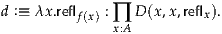 |
By path induction, we obtain apf : ∏(x,y:A) (x = y) → (f(x) = f(y)). The computation rule implies apf(reflx) ≡reflf(x) for each x : A. __
Second proof. By induction, it suffices to assume p is reflx. In this case, we may define apf(p) :≡reflf(x) : f(x) = f(x). __
We will often write apf(p) as simply f . This is strictly speaking
ambiguous, but generally no confusion arises. It matches the common
convention in category theory of using the same symbol for the application of
a functor to objects and to morphisms.
. This is strictly speaking
ambiguous, but generally no confusion arises. It matches the common
convention in category theory of using the same symbol for the application of
a functor to objects and to morphisms.
We note that ap behaves functorially, in all the ways that one might expect.
Proof. Left to the reader. __
As was the case for the equalities in Lemma 2.1.4, those in Lemma 2.2.2 are themselves paths, which satisfy their own coherence laws (which can be proved in the same way), and so on.
Since dependently typed functions are essential in type theory, we will also need a version of Lemma 2.2.1 for these. However, this is not quite so simple to state, because if f : ∏(x:A) B(x) and p : x = y, then f(x) : B(x) and f(y) : B(y) are elements of distinct types, so that a priori we cannot even ask whether they are equal. The missing ingredient is that p itself gives us a way to relate the types B(x) and B(y).
Lemma 2.3.1 (Transport). Suppose that P is a type family over A and that p : x =A y. Then there is a function p* : P(x) → P(y).
First proof. Let D : ∏(x,y:A) (x = y) → be the type family defined by
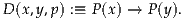
Then we have the function
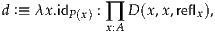 |
so that the induction principle gives us ind=A(D, d, x, y, p) : P(x) → P(y) for p : x = y, which we define to be p*. __
Second proof. By induction, it suffices to assume p is reflx. But in this case, we can take (reflx)* : P(x) → P(x) to be the identity function. __
Sometimes, it is necessary to notate the type family P in which the transport operation happens. In this case, we may write

Recall that a type family P over a type A can be seen as a property of elements of A, which holds at x in A if P(x) is inhabited. Then the transportation lemma says that P respects equality, in the sense that if x is equal to y, then P(x) holds if and only if P(y) holds. In fact, we will see later on that if x = y then actually P(x) and P(y) are equivalent.
Topologically, the transportation lemma can be viewed as a “path lifting”
operation in a fibration. We think of a type family P : A → as a fibration
with base space A, with P(x) being the fiber over x, and with ∑(x:A) P(x)
being the total space of the fibration, with first projection ∑(x:A) P(x) → A.
The defining property of a fibration is that given a path p : x = y in the
base space A and a point u : P(x) in the fiber over x, we may lift the
path p to a path in the total space starting at u (and this lifting can be
done continuously). The point p* can be thought of as the other
endpoint of this lifted path. We can also define the path itself in type
theory:
can be thought of as the other
endpoint of this lifted path. We can also define the path itself in type
theory:
Lemma 2.3.2 (Path lifting property). Let P : A →be a type family over A
and assume we have u : P(x) for some x : A. Then for any p : x = y, we
have
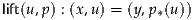 |
in ∑(x:A) P(x), such that pr1 = p.
= p.
Proof. Left to the reader. We will prove a more general theorem in §2.7. __
In classical homotopy theory, a fibration is defined as a map for which there exist liftings of paths; while in contrast, we have just shown that in type theory, every type family comes with a specified “path-lifting function”. This accords with the philosophy of constructive mathematics, according to which we cannot show that something exists except by exhibiting it. It also ensures automatically that the path liftings are chosen “continuously”, since as we have seen, all functions in type theory are “continuous”.
Remark 2.3.3. Although we may think of a type family P : A → as like
a fibration, it is generally not a good idea to say things like “the fibration
P : A →”, since this sounds like we are talking about a fibration with
base and total space A. To repeat, when a type family P : A → is
regarded as a fibration, the base is A and the total space is ∑(x:A) P(x).
We may also occasionally use other topological terminology when speaking about type families. For instance, we may refer to a dependent function f : ∏(x:A) P(x) as a section of the fibration P, and we may say that something happens fiberwise if it happens for each P(x). For instance, a section f : ∏(x:A) P(x) shows that P is “fiberwise inhabited”.
Now we can prove the dependent version of Lemma 2.2.1. The topological intuition is that given f : ∏(x:A) P(x) and a path p : x =A y, we ought to be able to apply f to p and obtain a path in the total space of P which “lies over” p, as shown below.
A ∑(x:A) P(x)pr 1xypf(x)f(y)f(p)
We can obtain such a thing from Lemma 2.2.1. Given f : ∏(x:A) P(x),
we can define a non-dependent function f′ : A → ∑(x:A) P(x) by
setting f′(x) :≡ (x, f(x)), and then consider f′ : f′(x) = f′(y). Since
pr1 ∘f′≡idA, by Lemma 2.2.2 we have pr1
: f′(x) = f′(y). Since
pr1 ∘f′≡idA, by Lemma 2.2.2 we have pr1 = p; thus f′
 does “lie
over” p in this sense. However, it is not obvious from the type of f′
does “lie
over” p in this sense. However, it is not obvious from the type of f′ that it
lies over any specific path in A (in this case, p), which is sometimes
important.
that it
lies over any specific path in A (in this case, p), which is sometimes
important.
The solution is to use the transport lemma. By Lemma 2.3.2 we have a
canonical path lift(u, p) from (x, u) to (y, p* ) which lies over p. Thus, any
path from u : P(x) to v : P(y) lying over p should factor through lift(u, p),
essentially uniquely, by a path from p*
) which lies over p. Thus, any
path from u : P(x) to v : P(y) lying over p should factor through lift(u, p),
essentially uniquely, by a path from p* to v lying entirely in the
fiber P(y). Thus, up to equivalence, it makes sense to define “a path
from u to v lying over p : x = y” to mean a path p*
to v lying entirely in the
fiber P(y). Thus, up to equivalence, it makes sense to define “a path
from u to v lying over p : x = y” to mean a path p* = v in P(y).
And, indeed, we can show that dependent functions produce such
paths.
= v in P(y).
And, indeed, we can show that dependent functions produce such
paths.
First proof. Let D : ∏(x,y:A) (x = y) → be the type family defined
by
 |
Then D(x, x, reflx) is (reflx)* = f(x). But since (reflx)*
 ≡ f(x),
we get that D(x, x, reflx) ≡ (f(x) = f(x)). Thus, we find the function
≡ f(x),
we get that D(x, x, reflx) ≡ (f(x) = f(x)). Thus, we find the function
 |
and now path induction gives us apdf(p) : p* = f(y) for each
p : x = y. __
= f(y) for each
p : x = y. __
Second proof. By induction, it suffices to assume p is reflx. But in
this case, the desired equation is (reflx)* ≡ f(x), which holds
judgmentally. __
≡ f(x), which holds
judgmentally. __
We will refer generally to paths which “lie over other paths” in this sense as dependent paths. They will play an increasingly important role starting in Chapter 6. In §2.5 we will see that for a few particular kinds of type families, there are equivalent ways to represent the notion of dependent paths that are sometimes more convenient.
Now recall from §1.4 that a non-dependently typed function f : A → B is just the special case of a dependently typed function f : ∏(x:A) P(x) when P is a constant type family, P(x) :≡ B. In this case, apdf and apf are closely related, because of the following lemma:
Lemma 2.3.5. If P : A →is defined by P(x) :≡ B for a fixed B : , then
for any x, y : Aand p : x = yand b : B we have a path

First proof. Fix a b : B, and let D : ∏(x,y:A) (x = y) → be the type
family defined by

Then D(x, x, reflx) is (transportP(reflx, b) = b), which is judgmentally equal to (b = b) by the computation rule for transporting. Thus, we have the function
Now path induction gives us an element of
 |
as desired. __
Second proof. By induction, it suffices to assume y is x and p is reflx. But transportP(reflx, b) ≡ b, so in this case what we have to prove is b = b, and we have reflb for this. __
Thus, for any x, y : A and p : x = y and f : A → B, by concatenating with transportconstB p(f(x)) and its inverse, respectively, we obtain functions
 f(x) = f(y) f(x) = f(y) | → p* p* = f(y) = f(y) and and | (2.3.6) |
 p* p* = f(y) = f(y) | → f(x) = f(y) f(x) = f(y) . . | (2.3.7) |
First proof. Let D : ∏(x,y:A) (x = y) → be the type family defined by

Thus, we have

But by definition, all three paths appearing in this type are reflf(x), so we have
Thus, path induction gives us an element of ∏(x,y:A) ∏(p:x=y) D(x, y, p), which is what we wanted. __
Second proof. By induction, it suffices to assume y is x and p is reflx. In this case, what we have to prove is reflf(x) = reflf(x) ▪reflf(x), which is true judgmentally. __
Because the types of apdf and apf are different, it is often clearer to use different notations for them.
At this point, we hope the reader is starting to get a feel for proofs by induction on identity types. From now on we stop giving both styles of proofs, allowing ourselves to use whatever is most clear and convenient (and often the second, more concise one). Here are a few other useful lemmas about transport; we leave it to the reader to give the proofs (in either style).
Lemma 2.3.10. For a function f : A → B and a type family P : B →, and
any p : x =A yand u : P(f(x)), we have

Lemma 2.3.11. For P, Q : A → and a family of functions f :
∏
(x:A) P(x) → Q(x), and any p : x =A yand u : P(x), we have

So far, we have seen how the identity type x =A y can be regarded as a type of identifications, paths, or equivalences between two elements x and y of a type A. Now we investigate the appropriate notions of “identification” or “sameness” between functions and between types. In §§2.9 and 2.10, we will see that homotopy type theory allows us to identify these with instances of the identity type, but before we can do that we need to understand them in their own right.
Traditionally, we regard two functions as the same if they take equal values on all inputs. Under the propositions-as-types interpretation, this suggests that two functions f and g (perhaps dependently typed) should be the same if the type ∏(x:A) (f(x) = g(x)) is inhabited. Under the homotopical interpretation, this dependent function type consists of continuous paths or functorial equivalences, and thus may be regarded as the type of homotopies or of natural isomorphisms.We will adopt the topological terminology for this.
Definition 2.4.1. Let f, g : ∏(x:A) P(x) be two sections of a type family
P : A →. A homotopy from f to g is a dependent function of type
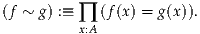 |
Note that a homotopy is not the same as an identification (f = g). However, in §2.9 we will introduce an axiom making homotopies and identifications “equivalent”.
The following proofs are left to the reader.
Lemma 2.4.2. Homotopy is an equivalence relation on each function type A → B. That is, we have elements of the types
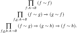
Just as functions in type theory are automatically “functors”, homotopies
are automatically “natural transformations”, in the following sense.
Recall that for f : A → B and p : x =A y, we may write f to mean
apf(p).
to mean
apf(p).
Lemma 2.4.3. Suppose H : f ~ gis a homotopy between functions f, g : A → B and let p : x =A y. Then we have
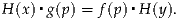 |
We may also draw this as a commutative diagram:
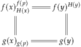 |
Proof. By induction, we may assume p is reflx. Since apf and apg compute on reflexivity, in this case what we must show is
But this follows since both sides are equal to H(x). __
Here f(x) denotes the ordinary application of f to x, while f denotes
apf(H(x)).
denotes
apf(H(x)).
Proof. By naturality of H, the following diagram of paths commutes:
 |
 ▪Hx = H(fx) ▪Hx. We can now whisker by (Hx)-1 to cancel
Hx, obtaining
▪Hx = H(fx) ▪Hx. We can now whisker by (Hx)-1 to cancel
Hx, obtaining

as desired (with some associativity paths suppressed). __
Of course, like the functoriality of functions (Lemma 2.2.2), the equality in Lemma 2.4.3 is a path which satisfies its own coherence laws, and so on.
Moving on to types, from a traditional perspective one may say that a function f : A → B is an isomorphism if there is a function g : B → A such that both composites f ∘g and g∘f are pointwise equal to the identity, i.e. such that f ∘g ~idB and g∘f ~idA. A homotopical perspective suggests that this should be called a homotopy equivalence, and from a categorical one, it should be called an equivalence of (higher) groupoids. However, when doing proof-relevant mathematics, the corresponding type
 | (2.4.5) |
is poorly behaved. For instance, for a single function f : A → B there may be multiple unequal inhabitants of (2.4.5). (This is closely related to the observation in higher category theory that often one needs to consider adjoint equivalences rather than plain equivalences.) For this reason, we give (2.4.5) the following historically accurate, but slightly derogatory-sounding name instead.
Definition 2.4.6. For a function f : A → B, a quasi-inverse of f is a triple (g, α, β) consisting of a function g : B → A and homotopies α : f ∘g ~idB and β : g∘f ~idA.
Thus, (2.4.5) is the type of quasi-inverses of f; we may denote it by qinv(f).
Example 2.4.7. The identity function idA : A → A has a quasi-inverse given by idA itself, together with homotopies defined by α(y) :≡ refly and β(x) :≡reflx.
Example 2.4.8. For any p : x =A y and z : A, the functions
| (p▪ –) | : (y =A z) → (x =A z) and | ||
| (– ▪p) | : (z =A x) → (z =A y) |
Example 2.4.9. For any p : x =A y and P : A →, the function
has a quasi-inverse given by transportP(p-1, –); this follows from
Lemma 2.3.9.
In general, we will only use the word isomorphism (and similar words such as bijection) in the special case when the types A and B “behave like sets” (see §3.1). In this case, the type (2.4.5) is unproblematic. We will reserve the word equivalence for an improved notion isequiv(f) with the following properties:
In Chapter 4 we will see that there are many different definitions of isequiv(f) which satisfy these three properties, but that all of them are equivalent. For now, to convince the reader that such things exist, we mention only the easiest such definition:
 | (2.4.10) |
We can show (i) and (ii) for this definition now. A function qinv(f) →isequiv(f) is easy to define by taking (g, α, β) to (g, α, g, β). In the other direction, given (g, α, h, β), let γ be the composite homotopy
and let β′ : g∘f ~idA be obtained from γ and β. Then (g, α, β′) : qinv(f).
Property (iii) for this definition is not too hard to prove either, but it requires identifying the identity types of cartesian products and dependent pair types, which we will discuss in §§2.6 and 2.7. Thus, we postpone it as well; see §4.3. At this point, the main thing to take away is that there is a well-behaved type which we can pronounce as “f is an equivalence”, and that we can prove f to be an equivalence by exhibiting a quasi-inverse to it. In practice, this is the most common way to prove that a function is an equivalence.
In accord with the proof-relevant philosophy, an equivalence from A to B is defined to be a function f : A → B together with an inhabitant of isequiv(f), i.e. a proof that it is an equivalence. We write (A ≃ B) for the type of equivalences from A to B, i.e. the type
 | (2.4.11) |
Property (iii) above will ensure that if two equivalences are equal as functions (that is, the underlying elements of A → B are equal), then they are also equal as equivalences (see §2.7). Thus, we often abuse notation by denoting an equivalence by the same letter as its underlying function.
We conclude by observing:
Lemma 2.4.12. Type equivalence is an equivalence relation on . More
specifically:
Proof. The identity function is clearly its own quasi-inverse; hence it is an equivalence.
If f : A → B is an equivalence, then it has a quasi-inverse, say f-1 : B → A. Then f is also a quasi-inverse of f-1, so f-1 is an equivalence B → A.
Finally, given f : A ≃ B and g : B ≃ C with quasi-inverses f-1 and g-1, say, then for any a : A we have f-1g-1gfa = f-1fa = a, and for any c : C we have gff-1g-1c = gg-1c = c. Thus f-1 ∘g-1 is a quasi-inverse to g∘f, hence the latter is an equivalence. __
In Chapter 1, we introduced many ways to form new types: cartesian products, disjoint unions, dependent products, dependent sums, etc. In §§2.1–2.3, we saw that all types in homotopy type theory behave like spaces or higher groupoids. Our goal in the rest of the chapter is to make explicit how this higher structure behaves in the case of the particular types defined in Chapter 1.
It turns out that for many types A, the equality types x =A y can be characterized, up to equivalence, in terms of whatever data was used to construct A. For example, if A is a cartesian product B×C, and x ≡ (b, c) and y ≡ (b′, c′), then we have an equivalence
 | (2.5.1) |
In more traditional language, two ordered pairs are equal just when their components are equal (but the equivalence (2.5.1) says rather more than this). The higher structure of the identity types can also be expressed in terms of these equivalences; for instance, concatenating two equalities between pairs corresponds to pairwise concatenation.
Similarly, when a type family P : A → is built up fiberwise using the
type forming rules from Chapter 1, the operation transportP(p, –) can be
characterized, up to homotopy, in terms of the corresponding operations on
the data that went into P. For instance, if P(x) ≡ B(x) ×C(x), then we
have

Finally, the type forming rules are also functorial, and if a function f is built from this functoriality, then the operations apf and apdf can be computed based on the corresponding ones on the data going into f. For instance, if g : B → B′ and h : C → C′ and we define f : B×C → B′×C′ by f(b, c) :≡ (g(b), h(c)), then modulo the equivalence (2.5.1), we can identify apf with “(apg, aph)”.
The next few sections (§§2.6–2.13) will be devoted to stating and proving theorems of this sort for all the basic type forming rules, with one section for each basic type former. Here we encounter a certain apparent deficiency in currently available type theories; as will become clear in later chapters, it would seem to be more convenient and intuitive if these characterizations of identity types, transport, and so on were judgmental equalities. However, in the theory presented in Chapter 1, the identity types are defined uniformly for all types by their induction principle, so we cannot “redefine” them to be different things at different types. Thus, the characterizations for particular types to be discussed in this chapter are, for the most part, theorems which we have to discover and prove, if possible.
Actually, the type theory of Chapter 1 is insufficient to prove the desired theorems for two of the type formers: Π-types and universes. For this reason, we are forced to introduce axioms into our type theory, in order to make those “theorems” true. Type-theoretically, an axiom (c.f. §1.1) is an “atomic” element that is declared to inhabit some specified type, without there being any rules governing its behavior other than those pertaining to the type it inhabits.
The axiom for Π-types (§2.9) is familiar to type theorists: it is called function extensionality, and states (roughly) that if two functions are homotopic in the sense of §2.4, then they are equal. The axiom for universes (§2.10), however, is a new contribution of homotopy type theory due to Voevodsky: it is called the univalence axiom, and states (roughly) that if two types are equivalent in the sense of §2.4, then they are equal. We have already remarked on this axiom in the introduction; it will play a very important role in this book.1
It is important to note that not all identity types can be “determined” by induction over the construction of types. Counterexamples include most nontrivial higher inductive types (see Chapters 6 and 8). For instance, calculating the identity types of the types Sn (see §6.4) is equivalent to calculating the higher homotopy groups of spheres, a deep and important field of research in algebraic topology.
Given types A and B, consider the cartesian product type A×B. For any
elements x, y : A×B and a path p : x =A×B y, by functoriality we can extract
paths pr1 : pr1(x) =A pr1(y) and pr2
 : pr2(x) =B pr2(y). Thus, we have
a function
: pr2(x) =B pr2(y). Thus, we have
a function
 | (2.6.1) |
Theorem 2.6.2. For any x and y, the function (2.6.1) is an equivalence.
Read logically, this says that two pairs are equal if they are equal componentwise. Read category-theoretically, this says that the morphisms in a product groupoid are pairs of morphisms. Read homotopy-theoretically, this says that the paths in a product space are pairs of paths.
Proof. We need a function in the other direction:
 | (2.6.3) |
By the induction rule for cartesian products, we may assume that x and y are both pairs, i.e. x ≡ (a, b) and y ≡ (a′, b′) for some a, a′ : A and b, b′ : B. In this case, what we want is a function
 |
Now by induction for the cartesian product in its domain, we may assume given p : a = a′ and q : b = b′. And by two path inductions, we may assume that a ≡ a′ and b ≡ b′ and both p and q are reflexivity. But in this case, we have (a, b) ≡ (a′, b′) and so we can take the output to also be reflexivity.
It remains to prove that (2.6.3) is quasi-inverse to (2.6.1). This is a simple sequence of inductions, but they have to be done in the right order.
In one direction, let us start with r : x =A×B y. We first do a path induction on r in order to assume that x ≡ y and r is reflexivity. In this case, since appr1 and appr2 are defined by path induction, (2.6.1) takes r ≡reflx to the pair (reflpr1x, reflpr2x). Now by induction on x, we may assume x ≡ (a, b), so that this is (refla, reflb). Thus, (2.6.3) takes it by definition to refl(a,b), which (under our current assumptions) is r.
In the other direction, if we start with s : (pr1(x) =A pr1(y)) × (pr2(x) =B pr2(y)), then we first do induction on x and y to assume that they are pairs (a, b) and (a′, b′), and then induction on s : (a =A a′) × (b =B b′) to reduce it to a pair (p, q) where p : a = a′ and q : b = b′. Now by induction on p and q, we may assume they are reflexivities refla and reflb, in which case (2.6.3) yields refl(a,b) and then (2.6.1) returns us to (refla, reflb) ≡ (p, q) ≡ s. __
In particular, we have shown that (2.6.1) has an inverse (2.6.3), which we may denote by

Note that a special case of this yields the propositional uniqueness principle for products: z = (pr1(z), pr2(z)).
It can be helpful to view pair= as a constructor or introduction rule for x = y, analogous to the “pairing” constructor of A×B itself, which introduces the pair (a, b) given a : A and b : B. From this perspective, the two components of (2.6.1):
| appr1 | : (x = y) → (pr1(x) = pr1(y)) | ||
| appr2 | : (x = y) → (pr2(x) = pr2(y)) |
| appr1 (pair=(p, q)) | = p for p : pr1x = pr1y | ||
| appr2 (pair=(p, q)) | = q for q : pr2x = pr2y |

We can also characterize the reflexivity, inverses, and composition of paths in A×B componentwise:
| refl(z:A×B) | = pair=(reflpr1z, reflpr2z) | ||
| p-1 | = pair= ap
pr1 (p)-1, ap
pr2 (p)-1 ap
pr1 (p)-1, ap
pr2 (p)-1 | ||
| p▪q | = pair= appr1 (p) ▪appr1 (q), appr2 (p) ▪appr2 (q) appr1 (p) ▪appr1 (q), appr2 (p) ▪appr2 (q) . . |
We now consider transport in a pointwise product of type families. Given
type families A, B : Z →, we abusively write A×B : Z → for the type
family defined by (A×B)(z) :≡ A(z) ×B(z). Now given p : z =Z w and
x : A(z) ×B(z), we can transport x along p to obtain an element of
A(w) ×B(w).
Proof. By path induction, we may assume p is reflexivity, in which case we have
| transportA×B(p, x) | ≡ x | ||
| transportA(p, pr1x) | ≡pr1x | ||
| transportB(p, pr2x) | ≡pr2x. |
Finally, we consider the functoriality of ap under cartesian products. Suppose given types A, B, A′, B′ and functions g : A → A′ and h : B → B′; then we can define a function f : A×B → A′×B′ by f(x) :≡ (g(pr1x), h(pr2x)).
Theorem 2.6.5. In the above situation, given x, y : A×B and p : pr1x = pr1yand q : pr2x = pr2y, we have

Proof. Note first that the above equation is well-typed. On the one hand,
since pair=(p, q) : x = y we have f : f(x) = f(y). On the
other hand, since pr1(f(x)) ≡ g(pr1x) and pr2(f(x)) ≡ h(pr2x), we also
have pair=(g
: f(x) = f(y). On the
other hand, since pr1(f(x)) ≡ g(pr1x) and pr2(f(x)) ≡ h(pr2x), we also
have pair=(g , h
, h ) : f(x) = f(y).
Now, by induction, we may assume x ≡ (a, b) and y ≡ (a′, b′), in which case we have p : a = a′ and q : b = b′. Thus, by path induction, we may assume p and q are reflexivity, in which case the desired equation holds judgmentally. __
Let A be a type and B : A → a type family. Recall that the Σ-type, or
dependent pair type, ∑(x:A) B(x) is a generalization of the cartesian
product type. Thus, we expect its higher groupoid structure to also be a
generalization of the previous section. In particular, its paths should be pairs
of paths, but it takes a little thought to give the correct types of these
paths.
Suppose that we have a path p : w = w′ in ∑(x:A) P(x). Then we get
pr1 : pr1(w) = pr1(w′). However, we cannot directly ask whether pr2(w) is
identical to pr2(w′) since they don’t have to be in the same type. But we can
transport pr2(w) along the path pr1
: pr1(w) = pr1(w′). However, we cannot directly ask whether pr2(w) is
identical to pr2(w′) since they don’t have to be in the same type. But we can
transport pr2(w) along the path pr1 , and this does give us an element of the
same type as pr2(w′). By path induction, we do in fact obtain a path
pr1
, and this does give us an element of the
same type as pr2(w′). By path induction, we do in fact obtain a path
pr1 *
* = pr2(w′).
Recall from the discussion preceding Lemma 2.3.4 that
 |
can be regarded as the type of paths from pr2(w) to pr2(w′) which lie over the
path pr1 in A. Thus, we are saying that a path w = w′ in the total space
determines (and is determined by) a path p : pr1(w) = pr1(w′) in A
together with a path from pr2(w) to pr2(w′) lying over p, which seems
sensible.
in A. Thus, we are saying that a path w = w′ in the total space
determines (and is determined by) a path p : pr1(w) = pr1(w′) in A
together with a path from pr2(w) to pr2(w′) lying over p, which seems
sensible.
Remark 2.7.1. Note that if we have x : A and u, v : P(x) such that
(x, u) = (x, v), it does not follow that u = v. All we can conclude is that
there exists p : x = x such that p* = v. This is a well-known source
of confusion for newcomers to type theory, but it makes sense from a
topological viewpoint: the existence of a path (x, u) = (x, v) in the total
space of a fibration between two points that happen to lie in the same
fiber does not imply the existence of a path u = v lying entirely within
that fiber.
= v. This is a well-known source
of confusion for newcomers to type theory, but it makes sense from a
topological viewpoint: the existence of a path (x, u) = (x, v) in the total
space of a fibration between two points that happen to lie in the same
fiber does not imply the existence of a path u = v lying entirely within
that fiber.
The next theorem states that we can also reverse this process. Since it is a direct generalization of Theorem 2.6.2, we will be more concise.
Theorem 2.7.2. Suppose that P : A →is a type family over a type Aand let
w, w′ : ∑(x:A) P(x). Then there is an equivalence
 |
Proof. We define for any w, w′ : ∑(x:A) P(x), a function
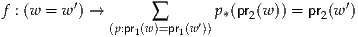 |
by path induction, with
 |
We want to show that f is an equivalence.
In the reverse direction, we define
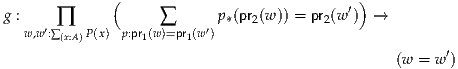
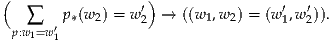 |
Next, given a pair ∑(p:w1=w′
1) p* = w2′, we can use Σ-induction
to get p : w1 = w1′ and q : p*
= w2′, we can use Σ-induction
to get p : w1 = w1′ and q : p* = w2′. Inducting on p, we have
q : refl*
= w2′. Inducting on p, we have
q : refl* = w2′, and it suffices to show (w1, w2) = (w1, w2′). But
refl*
= w2′, and it suffices to show (w1, w2) = (w1, w2′). But
refl* ≡ w2, so inducting on q reduces to the goal to (w1, w2) = (w1, w2),
which we can prove with refl(w1,w2).
≡ w2, so inducting on q reduces to the goal to (w1, w2) = (w1, w2),
which we can prove with refl(w1,w2).
Next we show that f(g(r)) = r for all w, w′ and r, where r has type
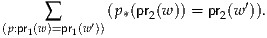
First, we break apart the pairs w, w′, and r by pair induction, as in the definition of g, and then use two path inductions to reduce both components of r to refl. Then it suffices to show that f(g(reflw1, reflw2)) = (reflw1, reflw2), which is true by definition.
Similarly, to show that g(f(p)) = p for all w, w′, and p : w = w′, we can do path induction on p, and then pair induction to split w, at which point it suffices to show that g(f(refl(w1,w2))) = refl(w1,w2), which is true by definition.
Thus, f has a quasi-inverse, and is therefore an equivalence. __
As we did in the case of cartesian products, we can deduce a propositional uniqueness principle as a special case.
Proof. We have reflpr1(z) : pr1(z) = pr1(pr1(z), pr2(z)), so by
Theorem 2.7.2 it will suffice to exhibit a path (reflpr1(z))* =
pr2(pr1(z), pr2(z)). But both sides are judgmentally equal to pr2(z). __
=
pr2(pr1(z), pr2(z)). But both sides are judgmentally equal to pr2(z). __
Like with binary cartesian products, we can think of the backward direction of Theorem 2.7.2 as an introduction form (pair=), the forward direction as elimination forms (appr1 and appr2 ), and the equivalence as giving a propositional computation rule and uniqueness principle for these.
Note that the lifted path lift(u, p) of p : x = y at u : P(x) defined in Lemma 2.3.2 may be identified with the special case of the introduction form

This appears in the statement of action of transport on Σ-types, which is also a generalization of the action for binary cartesian products:
Theorem 2.7.4. Suppose we have type families
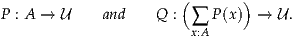 |
Then we can construct the type family over Adefined by
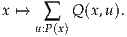 |
For any path p : x = yand any (u, z) : ∑(u:P(x)) Q(x, u) we have
 |
Proof. Immediate by path induction. __
We leave it to the reader to state and prove a generalization of Theorem 2.6.5 (see Exercise 2.7), and to characterize the reflexivity, inverses, and composition of Σ-types componentwise.
Trivial cases are sometimes important, so we mention briefly the case of the unit type 1.
It may be tempting to begin this proof by 1-induction on x and y, reducing the problem to (⋆ = ⋆) ≃1. However, at this point we would be stuck, since we would be unable to perform a path induction on p : ⋆ = ⋆. Thus, we instead work with a general x and y as much as possible, reducing them to ⋆ by induction only at the last moment.
Proof. A function (x = y) →1 is easy to define by sending everything to ⋆. Conversely, for any x, y : 1 we may assume by induction that x ≡ ⋆ ≡ y. In this case we have refl⋆ : x = y, yielding a constant function 1 → (x = y).
To show that these are inverses, consider first an element u : 1. We may assume that u ≡ ⋆, but this is also the result of the composite 1 → (x = y) →1.
On the other hand, suppose given p : x = y. By path induction, we may assume x ≡ y and p is reflx. We may then assume that x is ⋆, in which case the composite (x = y) → 1 → (x = y) takes p to reflx, i.e. to p. __
In particular, any two elements of 1 are equal. We leave it to the reader to formulate this equivalence in terms of introduction, elimination, computation, and uniqueness rules. The transport lemma for 1 is simply the transport lemma for constant type families (Lemma 2.3.5).
Given a type A and a type family B : A →, consider the dependent function
type ∏(x:A) B(x). We expect the type f = g of paths from f to g in ∏(x:A) B(x)
to be equivalent to the type of pointwise paths:
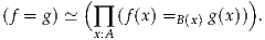 | (2.9.1) |
From a traditional perspective, this would say that two functions which are equal at each point are equal as functions. From a topological perspective, it would say that a path in a function space is the same as a continuous homotopy. And from a categorical perspective, it would say that an isomorphism in a functor category is a natural family of isomorphisms.
Unlike the case in the previous sections, however, the basic type theory presented in Chapter 1 is insufficient to prove (2.9.1). All we can say is that there is a certain function
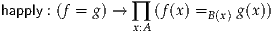 " class="math-display" >
 | (2.9.2) |
which is easily defined by path induction. For the moment, therefore, we will assume:
Axiom 2.9.3 (Function extensionality). For any A, B, f, and g, the function (2.9.2) is an equivalence.
We will see in later chapters that this axiom follows both from univalence (see §§2.10 and 4.9) and from an interval type (see §6.3 and Exercise 6.10).
In particular, Axiom 2.9.3 implies that (2.9.2) has a quasi-inverse
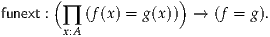
This function is also referred to as “function extensionality”. As we did with pair= in §2.6, we can regard funext as an introduction rule for the type f = g. From this point of view, happly is the elimination rule, while the homotopies witnessing funext as quasi-inverse to happly become a propositional computation rule

and a propositional uniqueness principle:

We can also compute the identity, inverses, and composition in Π-types; they are simply given by pointwise operations:.
| reflf | = funext(x reflf(x)) reflf(x)) | ||
| α-1 | = funext(x happly(α, x)-1) happly(α, x)-1) | ||
| α▪β | = funext(x happly(α, x) ▪happly(β, x)). happly(α, x) ▪happly(β, x)). |
Since the non-dependent function type A → B is a special case of the
dependent function type ∏(x:A) B(x) when B is independent of x, everything
we have said above applies in non-dependent cases as well. The rules for
transport, however, are somewhat simpler in the non-dependent case. Given a
type X, a path p : x1 =X x2, type families A, B : X →, and a function
f : A(x1) → B(x1), we have
| transportA→B(p, f) | =  x x transportB(p, f(transportA(p-1, x))) transportB(p, f(transportA(p-1, x))) | (2.9.4) |
defined by

In other words, when we transport a function f : A(x1) → B(x1) along a path p : x1 = x2, we obtain the function A(x2) → B(x2) which transports its argument backwards along p (in the type family A), applies f, and then transports the result forwards along p (in the type family B). This can be proven easily by path induction.
Transporting dependent functions is similar, but more complicated. Suppose
given X and p as before, type families A : X → and B : ∏(x:X) (A(x) →),
and also a dependent function f : ∏(a:A(x1)) B(x1, a). Then for a : A(x2), we
have
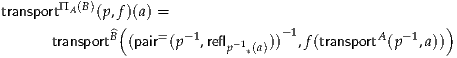
 denote respectively the type families
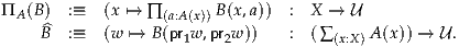 | (2.9.5) |
If these formulas look a bit intimidating, don’t worry about the details. The basic idea is just the same as for the non-dependent function type: we transport the argument backwards, apply the function, and then transport the result forwards again.
Now recall that for a general type family P : X →, in §2.2 we defined
the type of dependent paths over p : x =X y from u : P(x) to v : P(y)
to be p* =P(y) v. When P is a family of function types, there is
an equivalent way to represent this which is often more convenient.
=P(y) v. When P is a family of function types, there is
an equivalent way to represent this which is often more convenient.
Lemma 2.9.6. Given type families A, B : X →and p : x =X y, and also
f : A(x) → B(x) and g : A(y) → B(y), we have an equivalence
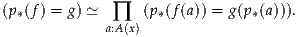
Moreover, if q : p* = g corresponds under this equivalence to
  , then for
a : A(x), the path
, then for
a : A(x), the path

is equal to the composite
(p* )(p* )(p* ) ) | = p* | (by (2.9.4)) | |
= p* | |||
= g(p* ). ). | (by  ) ) |
Proof. By path induction, we may assume p is reflexivity, in which case the desired equivalence reduces to function extensionality. The second statement then follows by the computation rule for function extensionality. __
As usual, the case of dependent functions is similar, but more complicated.
Lemma 2.9.7. Given type families A : X →and B : ∏(x:X) A(x) →
and p : x =X y, and also f : ∏(a:A(x)) B(x, a) and g : ∏(a:A(y)) B(y, a), we
have an equivalence

with  as in (2.9.5).
We leave it to the reader to prove this and to formulate a suitable computation rule.
Given two types A and B, we may consider them as elements of some
universe type , and thereby form the identity type A = B. As mentioned in
the introduction, univalence is the identification of A = B with the
type (A ≃ B) of equivalences from A to B, which we described in
§2.4. We perform this identification by way of the following canonical
function.
Proof. We could construct this directly by induction on equality, but the
following description is more convenient. Note that the identity function
id : → may be regarded as a type family indexed by the universe
; it assigns to each type X : the type X itself. (When regarded as
a fibration, its total space is the type ∑(A:) A of “pointed types”; see
also §4.8.) Thus, given a path p : A = B, we have a transport function
p* : A → B. We claim that p* is an equivalence. But by induction, it
suffices to assume that p is reflA, in which case p* ≡ idA, which is an
equivalence by Example 2.4.7. Thus, we can define idtoeqv(p) to be p*
(together with the above proof that it is an equivalence). __
We would like to say that idtoeqv is an equivalence. However, as with happly for function types, the type theory described in Chapter 1 is insufficient to guarantee this. Thus, as we did for function extensionality, we formulate this property as an axiom: Voevodsky’s univalence axiom.
Technically, the univalence axiom is a statement about a particular
universe type . If a universe satisfies this axiom, we say that it is
univalent. Except when otherwise noted (e.g. in §4.9) we will assume that all
universes are univalent.
Remark 2.10.4. It is important for the univalence axiom that we defined A ≃ B using a “good” version of isequiv as described in §2.4, rather than (say) as ∑(f:A→B) qinv(f). See Exercise 4.6.
In particular, univalence means that equivalent types may be identified. As we did in previous sections, it is useful to break this equivalence into:
B), denoted ua for “univalence
axiom”:


We can also identify the reflexivity, concatenation, and inverses of equalities in the universe with the corresponding operations on equivalences:
| reflA | = ua(idA) | ||
| ua(f) ▪ua(g) | = ua(g∘f) | ||
| ua(f)-1 | = ua(f-1). |

using Lemma 2.3.9 and the definition of idtoeqv. The third is similar.
The following observation, which is a special case of Lemma 2.3.10, is often useful when applying the univalence axiom.
Lemma 2.10.5. For any type family B : A →and x, y : Awith a path p : x = y
and u : B(x), we have
| transportB(p, u) | = transportX X(ap
B(p), u) X(ap
B(p), u) | ||
| = idtoeqv(apB(p))(u). |
Just as the type a =A a′ is characterized up to isomorphism, with a separate “definition” for each A, there is no simple characterization of the type p =a=Aa′ q of paths between paths p, q : a =A a′. However, our other general classes of theorems do extend to identity types, such as the fact that they respect equivalence.
Proof. Let f-1 be a quasi-inverse of f, with homotopies
 |
The quasi-inverse of apf is, essentially,

However, in order to obtain an element of a =A a′ from apf-1 (q), we must concatenate with the paths βa-1 and βa ′ on either side. To show that this gives a quasi-inverse of apf , on one hand we must show that for any p : a =A a′ we have
This follows from the functoriality of ap and the naturality of homotopies, Lemmas 2.2.2 and 2.4.3. On the other hand, we must show that for any q : f(a) =B f(a′) we have
The proof of this is a little more involved, but each step is again an application of Lemmas 2.2.2 and 2.4.3 (or simply canceling inverse paths):
apf | βa-1 ▪ap
f-1 (q) ▪βa′ | ||
= αf(a)-1 ▪α
f(a) ▪apf βa-1 ▪ap
f-1 (q) ▪βa′ βa-1 ▪ap
f-1 (q) ▪βa′ ▪αf(a′)-1 ▪α
f(a′) ▪αf(a′)-1 ▪α
f(a′) | |||
= αf(a)-1 ▪ap
f apf-1 apf-1  apf apf βa-1 ▪ap
f-1 (q) ▪βa′ βa-1 ▪ap
f-1 (q) ▪βa′   ▪αf(a′) ▪αf(a′) | |||
= αf(a)-1 ▪ap
f βa ▪βa-1 ▪ap
f-1 (q) ▪βa′▪βa′-1 βa ▪βa-1 ▪ap
f-1 (q) ▪βa′▪βa′-1 ▪α
f(a′) ▪α
f(a′) | |||
| = αf(a)-1 ▪ap f(apf-1 (q)) ▪αf(a′) | |||
| = q. | __
Thus, if for some type A we have a full characterization of a =A a′, the type p =a=Aa′ q is determined as well. For example:

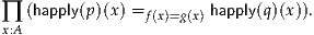
Next we consider transport in families of paths, i.e. transport in
C : A → where each C(x) is an identity type. The simplest case is
when C(x) is a type of paths in A itself, perhaps with one endpoint
fixed.
Lemma 2.11.2. For any Aand a : A, with p : x1 = x2, we have
transportx (a=x)(p, q) (a=x)(p, q) | = q▪p | for q : a = x1, | |||||
transportx (x=a)(p, q) (x=a)(p, q) | = p-1 ▪q | for q : x1 = a, | |||||
transportx (x=x)(p, q) (x=x)(p, q) | = p-1 ▪q▪p | for q : x1 = x1. |
Proof. Path induction on p, followed by the unit laws for composition. __
In other words, transporting with x c = x is post-composition, and
transporting with x
c = x is post-composition, and
transporting with x x = c is contravariant pre-composition. These may be
familiar as the functorial actions of the covariant and contravariant
hom-functors hom(c, –) and hom(–, c) in category theory.
x = c is contravariant pre-composition. These may be
familiar as the functorial actions of the covariant and contravariant
hom-functors hom(c, –) and hom(–, c) in category theory.
Similarly, we can prove the following more general form of Lemma 2.11.2, which is related to Lemma 2.3.10.
Because ap(x x) is the identity function and ap(x
 c) (where c is a constant)
is reflc, Lemma 2.11.2 is a special case. A yet more general version is when B
can be a family of types indexed on A:
c) (where c is a constant)
is reflc, Lemma 2.11.2 is a special case. A yet more general version is when B
can be a family of types indexed on A:
Theorem 2.11.4. Let B : A →and f, g : ∏(x:A) B(x), with p : a =A a′and
q : f(a) =B(a) g(a). Then we have
 |
Finally, as in §2.9, for families of identity types there is another equivalent characterization of dependent paths.
Proof. Path induction on p, followed by the fact that composing with the unit equalities q▪ 1 = q and r = 1 ▪r is an equivalence. __
There are more general equivalences involving the application of functions, akin to Theorems 2.11.3 and 2.11.4.
So far, most of the type formers we have considered have been what are called negative. Intuitively, this means that their elements are determined by their behavior under the elimination rules: a (dependent) pair is determined by its projections, and a (dependent) function is determined by its values. The identity types of negative types can almost always be characterized straightforwardly, along with all of their higher structure, as we have done in §§2.6–2.9. The universe is not exactly a negative type, but its identity types behave similarly: we have a straightforward characterization (univalence) and a description of the higher structure. Identity types themselves, of course, are a special case.
We now consider our first example of a positive type former. Again informally, a positive type is one which is “presented” by certain constructors, with the universal property of a presentation being expressed by its elimination rule. (Categorically speaking, a positive type has a “mapping out” universal property, while a negative type has a “mapping in” universal property.) Because computing with presentations is, in general, an uncomputable problem, for positive types we cannot always expect a straightforward characterization of the identity type. However, in many particular cases, a characterization or partial characterization does exist, and can be obtained by the general method that we introduce with this example.
(Technically, our chosen presentation of cartesian products and Σ-types is also positive. However, because these types also admit a negative presentation which differs only slightly, their identity types have a direct characterization that does not require the method to be described here.)
Consider the coproduct type A + B, which is “presented” by the injections inl : A → A + B and inr : B → A + B. Intuitively, we expect that A + B contains exact copies of A and B disjointly, so that we should have
| (inl(a1) = inl(a2)) | ≃ (a1 = a2) | (2.12.1) |
| (inr(b1) = inr(b2)) | ≃ (b1 = b2) | (2.12.2) |
| (inl(a) = inr(b)) | ≃0. | (2.12.3) |
 | (2.12.4) |
A similar argument would characterize the analogous family x (x = inr(b0))
for any b0 : B. Together, these characterizations imply (2.12.1)–(2.12.3).
(x = inr(b0))
for any b0 : B. Together, these characterizations imply (2.12.1)–(2.12.3).
In order to characterize (2.12.4), we will define a type family
code : A + B → and show that ∏(x:A+B) ((inl(a0) = x) ≃code(x)). Since we
want to conclude (2.12.1) from this, we should have code(inl(a)) = (a0 = a),
and since we also want to conclude (2.12.3), we should have code(inr(b)) = 0.
The essential insight is that we can use the recursion principle of A + B to
define code : A + B → by these two equations:
| code(inl(a)) | :≡ (a0 = a), | ||
| code(inr(b)) | :≡0. |
Proof. The key to the following proof is that we do it for all points x together, enabling us to use the elimination principle for the coproduct. We first define a function
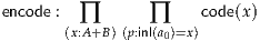
by transporting reflexivity along p:

Note that refla0 : code(inl(a0)), since code(inl(a0)) ≡ (a0 = a0) by definition of code. Next, we define a function
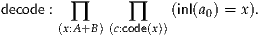
To define decode(x, c), we may first use the elimination principle of A + B to divide into cases based on whether x is of the form inl(a) or the form inr(b).
In the first case, where x ≡inl(a), then code(x) ≡ (a0 = a), so that c is an identification between a0 and a. Thus, apinl(c) : (inl(a0) = inl(a)) so we can define this to be decode(inl(a), c).
In the second case, where x ≡ inr(b), then code(x) ≡ 0, so that c inhabits the empty type. Thus, the elimination rule of 0 yields a value for decode(inr(b), c).
This completes the definition of decode; we now show that encode(x, –) and decode(x, –) are quasi-inverses for all x. On the one hand, suppose given x : A + B and p : inl(a0) = x; we want to show
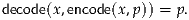 |
But now by (based) path induction, it suffices to consider x ≡inl(a0) and p ≡reflinl(a0):
| decode(x, encode(x, p)) | ≡decode(inl(a0), encode(inl(a0), reflinl(a0))) | ||
| ≡decode(inl(a0), transportcode(reflinl(a0), refla0)) | |||
| ≡decode(inl(a0), refla0) | |||
≡inl | |||
| ≡reflinl(a0) | |||
| ≡ p. |
| encode(x, decode(x, c)) | ≡transportcode(apinl(c), refla0) | ||
= transporta (a0=a)(c, refla
0) (a0=a)(c, refla
0) | (by Lemma 2.3.10) | ||
| = refla0 ▪c | (by Lemma 2.11.2) | ||
| = c. |
Of course, there is a corresponding theorem if we fix b0 : B instead of a0 : A.
In particular, Theorem 2.12.5 implies that for any a : A and b : B there are functions

and

The second of these states “inl(a0) is not equal to inr(b)”, i.e. the images of inl and inr are disjoint. The traditional reading of the first one, where identity types are viewed as propositions, is just injectivity of inl. The full homotopical statement of Theorem 2.12.5 gives more information: the types inl(a0) = inl(a) and a0 = a are actually equivalent, as are inr(b0) = inr(b) and b0 = b.
This proof illustrates a general method for describing path spaces, which we will use often. To characterize a path space, the first step is to define a comparison fibration “code” that provides a more explicit description of the paths. There are several different methods for proving that such a comparison fibration is equivalent to the paths (we show a few different proofs of the same result in §8.1). The one we have used here is called the encode-decode method: the key idea is to define decode generally for all instances of the fibration (i.e. as a function ∏ (x:A+B) code(x) → (inl(a0) = x)), so that path induction can be used to analyze decode(x, encode(x, p)).
As usual, we can also characterize the action of transport in coproduct
types. Given a type X, a path p : x1 =X x2, and type families A, B : X →,
we have
| transportA+B(p, inl(a)) | = inl(transportA(p, a)), | ||
| transportA+B(p, inr(b)) | = inr(transportB(p, b)), |
 A(x) + B(x). The proof is an easy path induction.
We use the encode-decode method to characterize the path space of the natural numbers, which are also a positive type. In this case, rather than fixing one endpoint, we characterize the two-sided path space all at once. Thus, the codes for identities are a type family
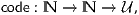
defined by double recursion over N as follows:
| code(0, 0) | :≡1 | ||
| code(succ(m), 0) | :≡0 | ||
| code(0, succ(n)) | :≡0 | ||
| code(succ(m), succ(n)) | :≡code(m, n). |
| r(0) | :≡ ⋆ | ||
| r(succ(n)) | :≡ r(n). |
Proof. We define
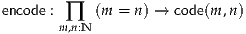
by transporting, encode(m, n, p) :≡transportcode(m, –)(p, r(m)). And we define
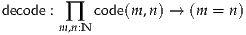
by double induction on m, n. When m and n are both 0, we need a function 1 → (0 = 0), which we define to send everything to refl0. When m is a successor and n is 0 or vice versa, the domain code(m, n) is 0, so the eliminator for 0 suffices. And when both are successors, we can define decode(succ(m), succ(n)) to be the composite
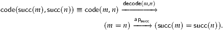
On one hand, if we start with p : m = n, then by induction on p it suffices to show

But encode(n, n, refln) ≡ r(n), so it suffices to show that decode(n, n, r(n)) = refln. We can prove this by induction on n. If n ≡ 0, then decode(0, 0, r(0)) = refl0 by definition of decode. And in the case of a successor, by the inductive hypothesis we have decode(n, n, r(n)) = refln, so it suffices to observe that apsucc(refln) ≡reflsucc(n).
On the other hand, if we start with c : code(m, n), then we proceed by double induction on m and n. If both are 0, then decode(0, 0, c) ≡refl0, while encode(0, 0, refl0) ≡ r(0) ≡ ⋆. Thus, it suffices to recall from §2.8 that every inhabitant of 1 is equal to ⋆. If m is 0 but n is a successor, or vice versa, then c : 0, so we are done. And in the case of two successors, we have
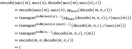 |
In particular, we have
 | (2.13.2) |
which shows that “0 is not the successor of any natural number”. We also have the composite
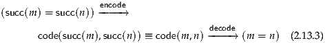
We will study more general positive types in Chapters 5 and 6. In Chapter 8, we will see that the same technique used here to characterize the identity types of coproducts and N can also be used to calculate homotopy groups of spheres.
We now consider one example to illustrate the interaction between the groupoid structure on a type and the type formers. In the introduction we remarked that one of the advantages of univalence is that two isomorphic things are interchangeable, in the sense that every property or construction involving one also applies to the other. Common “abuses of notation” become formally true. Univalence itself says that equivalent types are equal, and therefore interchangeable, which includes e.g. the common practice of identifying isomorphic sets. Moreover, when we define other mathematical objects as sets, or even general types, equipped with structure or properties, we can derive the correct notion of equality for them from univalence. We will illustrate this point with a significant example in Chapter 9, where we define the basic notions of category theory in such a way that equality of categories is equivalence, equality of functors is natural isomorphism, etc. See in particular §9.8. In this section, we describe a very simple example, coming from algebra.
For simplicity, we use semigroups as our example, where a semigroup is a type equipped with an associative “multiplication” operation. The same ideas apply to other algebraic structures, such as monoids, groups, and rings. Recall from §§1.6 and 1.11 that the definition of a kind of mathematical structure should be interpreted as defining the type of such structures as a certain iterated Σ-type. In the case of semigroups this yields the following.
Definition 2.14.1. Given a type A, the type SemigroupStr(A) of semigroup structures with carrier A is defined by

A semigroup is a type together with such a structure:
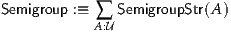
In the next two sections, we describe two ways in which univalence makes it easier to work with such semigroups.
When working loosely, one might say that a bijection between sets A and B “obviously” induces an isomorphism between semigroup structures on A and semigroup structures on B. With univalence, this is indeed obvious, because given an equivalence between types A and B, we can automatically derive a semigroup structure on B from one on A, and moreover show that this derivation is an equivalence of semigroup structures. The reason is that SemigroupStr is a family of types, and therefore has an action on paths between types given by transport:

Moreover, this map is an equivalence, because transportC(α) is always an equivalence with inverse transportC(α-1), see Lemmas 2.1.4 and 2.3.9.
While the univalence axiom ensures that this map exists, we need to use facts about transport proven in the preceding sections to calculate what it actually does. Let (m, a) be a semigroup structure on A, and we investigate the induced semigroup structure on B given by

First, because SemigroupStr(X) is defined to be a Σ-type, by Theorem 2.7.4,

where m′ is an induced multiplication operation on B
| m′ : B → B → B | |||
m′(b1, b2) :≡transportX (X→X→X)(ua(e), m)(b1, b2) (X→X→X)(ua(e), m)(b1, b2) |
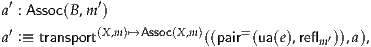 | (2.14.2) |
where Assoc(X, m) is the type ∏(x,y,z:X) m(x, m(y, z)) = m(m(x, y), z). By function extensionality, it suffices to investigate the behavior of m′ when applied to arguments b1, b2 : B. By applying (2.9.4) twice, we have that m′(b1, b2) is equal to
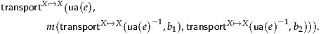
 X, this is equal to
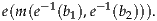
Thus, given two elements of B, the induced multiplication m′ sends them to A using the equivalence e, multiplies them in A, and then brings the result back to B by e, just as one would expect.
Moreover, though we do not show the proof, one can calculate that the induced proof that m′ is associative (see (2.14.2)) is equal to a function sending b1, b2, b3 : B to a path given by the following steps:
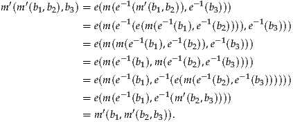 | (2.14.3) |
These steps use the proof a that m is associative and the inverse laws for e. From an algebra perspective, it may seem strange to investigate the identity of a proof that an operation is associative, but this makes sense if we think of A and B as general spaces, with non-trivial homotopies between paths. In Chapter 3, we will introduce the notion of a set, which is a type with only trivial homotopies, and if we consider semigroup structures on sets, then any two such associativity proofs are automatically equal.
Using the equations for path spaces discussed in the previous sections, we can investigate when two semigroups are equal. Given semigroups (A, m, a) and (B, m′, a′), by Theorem 2.7.2, the type of paths
 |
is equal to the type of pairs
| p1 | : A = B and | ||
| p2 | : transportSemigroupStr(p1, (m, a)) = (m′, a′). |
 |
and the second of which shows that a′ is equal to the induced associativity proof constructed from a in (2.14.3). But by cancellation of inverses (2.14.2) is equivalent to
This says that e commutes with the binary operation, in the sense that it takes multiplication in A (i.e. m) to multiplication in B (i.e. m′). A similar rearrangement is possible for the equation relating a and a′. Thus, an equality of semigroups consists exactly of an equivalence on the carrier types that commutes with the semigroup structure.
For general types, the proof of associativity is thought of as part of the structure of a semigroup. However, if we restrict to set-like types (again, see Chapter 3), the equation relating a and a′ is trivially true. Moreover, in this case, an equivalence between sets is exactly a bijection. Thus, we have arrived at a standard definition of a semigroup isomorphism: a bijection on the carrier sets that preserves the multiplication operation. It is also possible to use the category-theoretic definition of isomorphism, by defining a semigroup homomorphism to be a map that preserves the multiplication, and arrive at the conclusion that equality of semigroups is the same as two mutually inverse homomorphisms; but we will not show the details here; see §9.8.
The conclusion is that, thanks to univalence, semigroups are equal precisely when they are isomorphic as algebraic structures. As we will see in §9.8, the conclusion applies more generally: in homotopy type theory, all constructions of mathematical structures automatically respect isomorphisms, without any tedious proofs or abuse of notation.
By combining the path computation rules described in the preceding sections, we can show that various type forming operations satisfy the expected universal properties, interpreted in a homotopical way as equivalences. For instance, given types X, A, B, we have a function
 | (2.15.1) |
defined by f (pr1 ∘f, pr2 ∘f).
Theorem 2.15.2. (2.15.1) is an equivalence.
Proof. We define the quasi-inverse by sending (g, h) to λx.(g(x), h(x)). (Technically, we have used the induction principle for the cartesian product (X → A) × (X → B), to reduce to the case of a pair. From now on we will often apply this principle without explicit mention.)
Now given f : X → A×B, the round-trip composite yields the function
 | (2.15.3) |
By Theorem 2.6.2, for any x : X we have (pr1(f(x)), pr2(f(x))) = f(x). Thus, by function extensionality, the function (2.15.3) is equal to f.
On the other hand, given (g, h), the round-trip composite yields the pair (λx.g(x), λx.h(x)). By the uniqueness principle for functions, this is (judgmentally) equal to (g, h). __
In fact, we also have a dependently typed version of this universal
property. Suppose given a type X and type families A, B : X →. Then we
have a function
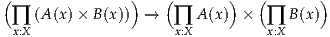 | (2.15.4) |
defined as before by f (pr1 ∘f, pr2 ∘f).
Theorem 2.15.5. (2.15.4) is an equivalence.
Proof. Left to the reader. __
Just as Σ-types are a generalization of cartesian products, they
satisfy a generalized version of this universal property. Jumping right to
the dependently typed version, suppose we have a type X and type
families A : X → and P : ∏(x:X) A(x) →. Then we have a function
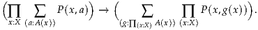 | (2.15.6) |
Note that if we have P(x, a) :≡ B(x) for some B : X →, then (2.15.6)
reduces to (2.15.4).
Theorem 2.15.7. (2.15.6) is an equivalence.
Proof. As before, we define a quasi-inverse to send (g, h) to the function λx.(g(x), h(x)). Now given f : ∏(x:X) ∑(a:A(x)) P(x, a), the round-trip composite yields the function
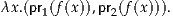 | (2.15.8) |
Now for any x : X, by Corollary 2.7.3 (the uniqueness principle for Σ-types) we have
 |
Thus, by function extensionality, (2.15.8) is equal to f. On the other hand, given (g, h), the round-trip composite yields (λx.g(x), λx.h(x)), which is judgmentally equal to (g, h) as before. __
This is noteworthy because the propositions-as-types interpretation of (2.15.6) is “the axiom of choice”. If we read Σ as “there exists” and Π (sometimes) as “for all”, we can pronounce:
Thus, Theorem 2.15.7 says that not only is the axiom of choice “true”, its antecedent is actually equivalent to its conclusion. (On the other hand, the classical mathematician may find that (2.15.6) does not carry the usual meaning of the axiom of choice, since we have already specified the values of g, and there are no choices left to be made. We will return to this point in §3.8.)
The above universal property for pair types is for “mapping in”, which is familiar from the category-theoretic notion of products. However, pair types also have a universal property for “mapping out”, which may look less familiar. In the case of cartesian products, the non-dependent version simply expresses the cartesian closure adjunction:

The dependent version of this is formulated for a type family C : A×B →:
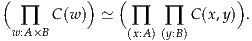
Here the right-to-left function is simply the induction principle for A×B, while the left-to-right is evaluation at a pair. We leave it to the reader to prove that these are quasi-inverses. There is also a version for Σ-types:
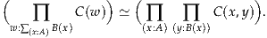 | (2.15.9) |
Again, the right-to-left function is the induction principle.
Some other induction principles are also part of universal properties of this sort. For instance, path induction is the right-to-left direction of an equivalence as follows:
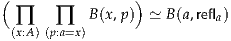 | (2.15.10) |
for any a : A and type family B : ∏(x:A) (a = x) →. However, inductive
types with recursion, such as the natural numbers, have more complicated
universal properties; see Chapter 5.
Since Theorem 2.15.2 expresses the usual universal property of a cartesian product (in an appropriate homotopy-theoretic sense), the categorically inclined reader may well wonder about other limits and colimits of types. In Exercise 2.9 we ask the reader to show that the coproduct type A + B also has the expected universal property, and the nullary cases of 1 (the terminal object) and 0 (the initial object) are easy.
For pullbacks, the expected explicit construction works: given f : A → C and g : B → C, we define
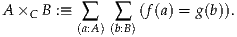 | (2.15.11) |
In Exercise 2.11 we ask the reader to verify this. Some more general homotopy limits can be constructed in a similar way, but for colimits we will need a new ingredient; see Chapter 6.
The definition of identity types, with their induction principle, is due to Martin-Löf [ML98]. As mentioned in the notes to Chapter 1, our identity types are those that belong to intensional type theory, rather than extensional type theory. In general, a notion of equality is said to be “intensional” if it distinguishes objects based on their particular definitions, and “extensional” if it does not distinguish between objects that have the same “extension” or “observable behavior”. In the terminology of Frege, an intensional equality compares sense, while an extensional one compares only reference. We may also speak of one equality being “more” or “less” extensional than another, meaning that it takes account of fewer or more intensional aspects of objects, respectively.
Intensional type theory is so named because its judgmental equality, x ≡ y, is a very intensional equality: it says essentially that x and y “have the same definition”, after we expand the defining equations of functions. By contrast, the propositional equality type x = y is more extensional, even in the axiom-free intensional type theory of Chapter 1: for instance, we can prove by induction that n + m = m + n for all m, n : N, but we cannot say that n + m ≡ m + n for all m, n : N, since the definition of addition treats its arguments asymmetrically. We can make the identity type of intensional type theory even more extensional by adding axioms such as function extensionality (two functions are equal if they have the same behavior on all inputs, regardless of how they are defined) and univalence (which can be regarded as an extensionality property for the universe: two types are equal if they behave the same in all contexts). The axioms of function extensionality, and univalence in the special case of mere propositions (“propositional extensionality”), appeared already in the first type theories of Russell and Church.
As mentioned before, extensional type theory includes also a “reflection rule” saying that if p : x = y, then in fact x ≡ y. Thus extensional type theory is so named because it does not admit any purely intensional equality: the reflection rule forces the judgmental equality to coincide with the more extensional identity type. Moreover, from the reflection rule one may deduce function extensionality (at least in the presence of a judgmental uniqueness principle for functions). However, the reflection rule also implies that all the higher groupoid structure collapses (see Exercise 2.14), and hence is inconsistent with the univalence axiom (see Example 3.1.9). Therefore, regarding univalence as an extensionality property, one may say that intensional type theory permits identity types that are “more extensional” than extensional type theory does.
The proofs of symmetry (inversion) and transitivity (concatenation) for equalities are well-known in type theory. The fact that these make each type into a 1-groupoid (up to homotopy) was exploited in [HS98] to give the first “homotopy” style semantics for type theory.
The actual homotopical interpretation, with identity types as path spaces, and type families as fibrations, is due to [AW09], who used the formalism of Quillen model categories. An interpretation in (strict) ∞-groupoids was also given in the thesis [War08]. For a construction of all the higher operations and coherences of an ∞-groupoid in type theory, see [Lum10] and [vdBG11].
Operations such as transportP(p, –) and apf , and one good notion of equivalence, were first studied extensively in type theory by Voevodsky, using the proof assistant Coq. Subsequently, many other equivalent definitions of equivalence have been found, which are compared in Chapter 4.
The “computational” interpretation of identity types, transport, and so on described in §2.5 has been emphasized by [LH12]. They also described a “1-truncated” type theory (see Chapter 7) in which these rules are judgmental equalities. The possibility of extending this to the full untruncated theory is a subject of current research.
The naive form of function extensionality which says that “if two functions are pointwise equal, then they are equal” is a common axiom in type theory, going all the way back to [WR27]. Some stronger forms of function extensionality were considered in [Gar09]. The version we have used, which identifies the identity types of function types up to equivalence, was first studied by Voevodsky, who also proved that it is implied by the naive version (and by univalence; see §4.9).
The univalence axiom is also due to Voevodsky. It was originally motivated by semantic considerations in the simplicial set model; see [KLV12]. A similar axiom motivated by the groupoid model was proposed by Hofmann and Streicher [HS98] under the name “universe extensionality”. It used quasi-inverses (2.4.5) rather than a good notion of “equivalence”, and hence is correct (and equivalent to univalence) only for a universe of 1-types (see Definition 3.1.7).
In the type theory we are using in this book, function extensionality and univalence have to be assumed as axioms, i.e. elements asserted to belong to some type but not constructed according to the rules for that type. While serviceable, this has a few drawbacks. For instance, type theory is formally better-behaved if we can base it entirely on rules rather than asserting axioms. It is also sometimes inconvenient that the theorems of §§2.6–2.13 are only propositional equalities (paths) or equivalences, since then we must explicitly mention whenever we pass back and forth across them. One direction of current research in homotopy type theory is to describe a type system in which these rules are judgmental equalities, solving both of these problems at once. So far this has only been done in some simple cases, although preliminary results such as [LH12] are promising. There are also other potential ways to introduce univalence and function extensionality into a type theory, such as having a sufficiently powerful notion of “higher quotients” or “higher inductive-recursive types”.
The simple conclusions in §§2.12–2.13 such as “inl and inr are injective and disjoint” are well-known in type theory, and the construction of the function encode is the usual way to prove them. The more refined approach we have described, which characterizes the entire identity type of a positive type (up to equivalence), is a more recent development; see e.g. [LS13a].
The type-theoretic axiom of choice (2.15.6) was noticed in William Howard’s original paper [How80] on the propositions-as-types correspondence, and was studied further by Martin-Löf with the introduction of his dependent type theory. It is mentioned as a “distributivity law” in Bourbaki’s set theory [Bou68].
For a more comprehensive (and formalized) discussion of pullbacks and more general homotopy limits in homotopy type theory, see [AKL13]. Limits of diagrams over directed graphs are the easiest general sort of limit to formalize; the problem with diagrams over categories (or more generally (∞, 1)-categories) is that in general, infinitely many coherence conditions are involved in the notion of (homotopy coherent) diagram. Resolving this problem is an important open question in homotopy type theory.
Exercise 2.1. Show that the three obvious proofs of Lemma 2.1.2 are pairwise equal.
Exercise 2.2. Show that the three equalities of proofs constructed in the previous exercise form a commutative triangle. In other words, if the three definitions of concatenation are denoted by (p ▪1 q), (p ▪2 q), and (p ▪3 q), then the concatenated equality

is equal to the equality (p ▪1 q) = (p ▪3 q).
Exercise 2.3. Give a fourth, different, proof of Lemma 2.1.2, and prove that it is equal to the others.
Exercise 2.4. Define, by induction on n, a general notion of n-dimensional path in a type A, simultaneously with the type of boundaries for such paths.
Exercise 2.6. Prove that if p : x = y, then the function (p▪ –) : (y = z) → (x = z) is an equivalence.
Exercise 2.7. State and prove a generalization of Theorem 2.6.5 from cartesian products to Σ-types.
Exercise 2.8. State and prove an analogue of Theorem 2.6.5 for coproducts.
Exercise 2.9. Prove that coproducts have the expected universal property,

Can you generalize this to an equivalence involving dependent functions?
Exercise 2.10. Prove that Σ-types are “associative”, in that for any A :
and families B : A → and C : ( ∑(x:A) B(x)) →, we have
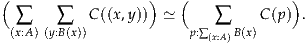
Exercise 2.11. A (homotopy) commutative square
 |
consists of functions f, g, h, and k as shown, together with a path f ∘h = g∘k. Note that this is exactly an element of the pullback (P → A) ×P→C(P → B) as defined in (2.15.11). A commutative square is called a (homotopy) pullback square if for any X, the induced map

is an equivalence. Prove that the pullback P :≡ A×CB defined in (2.15.11) is the corner of a pullback square.
Exercise 2.12. Suppose given two commutative squares
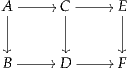 |
and suppose that the right-hand square is a pullback square. Prove that the left-hand square is a pullback square if and only if the outer rectangle is a pullback square.
Exercise 2.14. Suppose we add to type theory the equality reflection rule which says that if there is an element p : x = y, then in fact x ≡ y. Prove that for any p : x = x we have p ≡reflx. (This implies that every type is a set in the sense to be introduced in §3.1; see §7.2.)
Exercise 2.15. Show that Lemma 2.10.5 can be strengthened to

without using function extensionality. (In this and other similar cases, the apparently weaker formulation has been chosen for readability and consistency.)
Exercise 2.16. Suppose that rather than function extensionality (Axiom 2.9.3), we suppose only the existence of an element
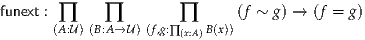
(with no relationship to happly assumed). Prove that in fact, this is sufficient to imply the whole function extensionality axiom (that happly is an equivalence). This is due to Voevodsky; its proof is tricky and may require concepts from later chapters.
Type theory, formal or informal, is a collection of rules for manipulating types and their elements. But when writing mathematics informally in natural language, we generally use familiar words, particularly logical connectives such as “and” and “or”, and logical quantifiers such as “for all” and “there exists”. In contrast to set theory, type theory offers us more than one way to regard these English phrases as operations on types. This potential ambiguity needs to be resolved, by setting out local or global conventions, by introducing new annotations to informal mathematics, or both. This requires some getting used to, but is offset by the fact that because type theory permits this finer analysis of logic, we can represent mathematics more faithfully, with fewer “abuses of language” than in set-theoretic foundations. In this chapter we will explain the issues involved, and justify the choices we have made.
In order to explain the connection between the logic of type theory and the logic of set theory, it is helpful to have a notion of set in type theory. While types in general behave like spaces or higher groupoids, there is a subclass of them that behave more like the sets in a traditional set-theoretic system. Categorically, we may consider discrete groupoids, which are determined by a set of objects and only identity morphisms as higher morphisms; while topologically, we may consider spaces having the discrete topology. More generally, we may consider groupoids or spaces that are equivalent to ones of this sort; since everything we do in type theory is up to homotopy, we can’t expect to tell the difference.
Intuitively, we would expect a type to “be a set” in this sense if it has no higher homotopical information: any two parallel paths are equal (up to homotopy), and similarly for parallel higher paths at all dimensions. Fortunately, because everything in homotopy type theory is automatically functorial/continuous, it turns out to be sufficient to ask this at the bottom level.
More precisely, the proposition isSet(A) is defined to be the type
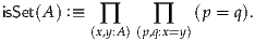
As mentioned in §1.1, the sets in homotopy type theory are not like the sets in ZF set theory, in that there is no global “membership predicate” ∈. They are more like the sets used in structural mathematics and in category theory, whose elements are “abstract points” to which we give structure with functions and relations. This is all we need in order to use them as a foundational system for most set-based mathematics; we will see some examples in Chapter 10.
Which types are sets? In Chapter 7 we will study a more general form of this question in depth, but for now we can observe some easy examples.
Example 3.1.2. The type 1 is a set. For by Theorem 2.8.1, for any x, y : 1 the type (x = y) is equivalent to 1. Since any two elements of 1 are equal, this implies that any two elements of x = y are equal.
Example 3.1.3. The type 0 is a set, for given any x, y : 0 we may deduce anything we like, by the induction principle of 0.
Example 3.1.4. The type N of natural numbers is also a set. This follows from Theorem 2.13.1, since all equality types x =N y are equivalent to either 1 or 0, and any two inhabitants of 1 or 0 are equal. We will see another proof of this fact in Chapter 7.
Most of the type forming operations we have considered so far also preserve sets.
Example 3.1.5. If A and B are sets, then so is A×B. For given x, y : A×B and p, q : x = y, by Theorem 2.6.2 we have p = pair=(appr1 (p), appr2 (p)) and q = pair=(appr1 (q), appr2 (q)). But appr1 (p) = appr1 (q) since A is a set, and appr2 (p) = appr2 (q) since B is a set; hence p = q.
Similarly, if A is a set and B : A → is such that each B(x) is a set,
then ∑(x:A) B(x) is a set.
Example 3.1.6. If A is any type and B : A → is such that each B(x) is a set,
then the type ∏(x:A) B(x) is a set. For suppose f, g : ∏(x:A) B(x) and
p, q : f = g. By function extensionality, we have
 |
But for any x : A, we have
 |
so since B(x) is a set we have happly(p, x) = happly(q, x). Now using function
extensionality again, the dependent functions (x happly(p, x)) and
(x
happly(p, x)) and
(x happly(q, x)) are equal, and hence (applying apfunext) so are p
and q.
happly(q, x)) are equal, and hence (applying apfunext) so are p
and q.
For more examples, see Exercises 3.2 and 3.3. For a more systematic investigation of the subsystem (category) of all sets in homotopy type theory, see Chapter 10.
Sets are just the first rung on a ladder of what are called homotopy n-types. The next rung consists of 1-types, which are analogous to 1-groupoids in category theory. The defining property of a set (which we may also call a 0-type) is that it has no non-trivial paths. Similarly, the defining property of a 1-type is that it has no non-trivial paths between paths:
Definition 3.1.7. A type A is a 1-type if for all x, y : A and p, q : x = y and r, s : p = q, we have r = s.
Similarly, we can define 2-types, 3-types, and so on. We will define the general notion of n-type inductively in Chapter 7, and study the relationships between them.
However, for now it is useful to have two facts in mind. First, the levels are upward-closed: if A is an n-type then A is an (n + 1)-type. For example:
Proof. Suppose f : isSet(A); then for any x, y : A and p, q : x = y we have
f(x, y, p, q) : p = q. Fix x, y, and p, and define g : ∏(q:x=y) (p = q) by
g(q) :≡ f(x, y, p, q). Then for any r : q = q′, we have apdg(r) : r* =
g(q′). By Lemma 2.11.2, therefore, we have g(q) ▪r = g(q′).
=
g(q′). By Lemma 2.11.2, therefore, we have g(q) ▪r = g(q′).
In particular, suppose given x, y, p, q and r, s : p = q, as in Definition 3.1.7, and define g as above. Then g(p) ▪r = g(q) and also g(p) ▪s = g(q), hence by cancellation r = s. __
Second, this stratification of types by level is not degenerate, in the sense that not all types are sets:
Example 3.1.9. The universe is not a set. To prove this, it suffices to
exhibit a type A and a path p : A = A which is not equal to reflA.
Take A = 2, and let f : A → A be defined by f(02) :≡ 12 and
f(12) :≡ 02. Then f(f(x)) = x for all x (by an easy case analysis), so f is
an equivalence. Hence, by univalence, f gives rise to a path p : A = A.
If p were equal to reflA, then (again by univalence) f would equal the identity function of A. But this would imply that 02 = 12, contradicting Remark 2.12.6.
In Chapters 6 and 8 we will show that for any n, there are types which are not n-types.
Note that A is a 1-type exactly when for any x, y : A, the identity type x =A y is a set. (Thus, Lemma 3.1.8 could equivalently be read as saying that the identity types of a set are also sets.) This will be the basis of the recursive definition of n-types we will give in Chapter 7.
We can also extend this characterization “downwards” from sets. That is, a type A is a set just when for any x, y : A, any two elements of x =A y are equal. Since sets are equivalently 0-types, it is natural to call a type a (-1)-type if it has this latter property (any two elements of it are equal). Such types may be regarded as propositions in a narrow sense, and their study is just what is usually called “logic”; it will occupy us for the rest of this chapter.
Until now, we have been following the straightforward “propositions as types” philosophy described in §1.11, according to which English phrases such as “there exists an x : A such that P(x)” are interpreted by corresponding types such as ∑(x:A) P(x), with the proof of a statement being regarded as judging some specific element to inhabit that type. However, we have also seen some ways in which the “logic” resulting from this reading seems unfamiliar to a classical mathematician. For instance, in Theorem 2.15.7 we saw that the statement
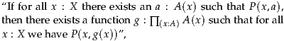 | (3.2.1) |
which looks like the classical axiom of choice, is always true under this reading. This is a noteworthy, and often useful, feature of the propositions-as-types logic, but it also illustrates how significantly it differs from the classical interpretation of logic, under which the axiom of choice is not a logical truth, but an additional “axiom”.
On the other hand, we can now also show that corresponding statements looking like the classical law of double negation and law of excluded middle are incompatible with the univalence axiom.
Proof. Recall that ¬A ≡ (A → 0). We also read “it is not the case that
…” as the operator ¬. Thus, in order to prove this statement, it suffices to
assume given some f : ∏(A:) (¬¬A → A) and construct an element of
0.
The idea of the following proof is to observe that f, like any function in type theory, is “continuous”. By univalence, this implies that f is natural with respect to equivalences of types. From this, and a fixed-point-free autoequivalence, we will be able to extract a contradiction.
Let e : 2 ≃ 2 be the equivalence defined by e(12) :≡ 02 and e(02) :≡ 12, as in Example 3.1.9. Let p : 2 = 2 be the path corresponding to e by univalence, i.e. p :≡ua(e). Then we have f(2) : ¬¬2 →2 and

Hence, for any u : ¬¬2, we have

Now by (2.9.4), transporting f(2) : ¬¬2 →2 along p in the type family
A (¬¬A → A) is equal to the function which transports its argument along
p-1 in the type family A
(¬¬A → A) is equal to the function which transports its argument along
p-1 in the type family A ¬¬A, applies f(2), then transports the result along
p in the type family A
¬¬A, applies f(2), then transports the result along
p in the type family A A:
A:
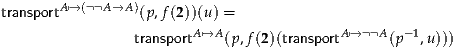
 ¬¬A(p-1, u) = u, and so
from happly(apdf
¬¬A(p-1, u) = u, and so
from happly(apdf , u) we obtain an equality

Finally, as discussed in §2.10, transporting in the type family A A along the
path p ≡ua(e) is equivalent to applying the equivalence e; thus we
have
A along the
path p ≡ua(e) is equivalent to applying the equivalence e; thus we
have
 | (3.2.3) |
However, we can also prove that
 | (3.2.4) |
This follows from a case analysis on x: both cases are immediate from the definition of e and the fact that 02≠12 (Remark 2.12.6). Thus, applying (3.2.4) to f(2)(u) and (3.2.3), we obtain an element of 0. __
Remark 3.2.5. In particular, this implies that there can be no Hilbert-style “choice operator” which selects an element of every nonempty type. The point is that no such operator can be natural, and under the univalence axiom, all functions acting on types must be natural with respect to equivalences.
Remark 3.2.6. It is, however, still the case that ¬¬¬A →¬A for any A; see Exercise 1.11.
Proof. Suppose we had g : ∏(A:) (A + (¬A)). We will show that then
∏
(A:) (¬¬A → A), so that we can apply Theorem 3.2.2. Thus, suppose
A : and u : ¬¬A; we want to construct an element of A.
Now g(A) : A + (¬A), so by case analysis, we may assume either g(A) ≡inl(a) for some a : A, or g(A) ≡inr(w) for some w : ¬A. In the first case, we have a : A, while in the second case we have u(w) : 0 and so we can obtain anything we wish (such as A). Thus, in both cases we have an element of A, as desired. __
Thus, if we want to assume the univalence axiom (which, of course, we do) and still leave ourselves the option of classical reasoning (which is also desirable), we cannot use the unmodified propositions-as-types principle to interpret all informal mathematical statements into type theory, since then the law of excluded middle would be false. However, neither do we want to discard propositions-as-types entirely, because of its many good properties (such as simplicity, constructivity, and computability). We now discuss a modification of propositions-as-types which resolves these problems; in §3.10 we will return to the question of which logic to use when.
We have seen that the propositions-as-types logic has both good and bad properties. Both have a common cause: when types are viewed as propositions, they can contain more information than mere truth or falsity, and all “logical” constructions on them must respect this additional information. This suggests that we could obtain a more conventional logic by restricting attention to types that do not contain any more information than a truth value, and only regarding these as logical propositions.
Such a type A will be “true” if it is inhabited, and “false” if its inhabitation yields a contradiction (i.e. if ¬A ≡ (A →0) is inhabited). What we want to avoid, in order to obtain a more traditional sort of logic, is treating as logical propositions those types for which giving an element of them gives more information than simply knowing that the type is inhabited. For instance, if we are given an element of 2, then we receive more information than the mere fact that 2 contains some element. Indeed, we receive exactly one bit more information: we know which element of 2 we were given. By contrast, if we are given an element of 1, then we receive no more information than the mere fact that 1 contains an element, since any two elements of 1 are equal to each other. This suggests the following definition.
Note that since we are still doing mathematics in type theory, this is
a definition in type theory, which means it is a type — or, rather, a
type family. Specifically, for any P : , the type isProp(P) is defined to
be
Thus, to assert that “P is a mere proposition” means to exhibit an inhabitant of isProp(P), which is a dependent function connecting any two elements of P by a path. The continuity/naturality of this function implies that not only are any two elements of P equal, but P contains no higher homotopy either.
Proof. Define f : P →1 by f(x) :≡ ⋆, and g : 1 → P by g(u) :≡ x0. The claim follows from the next lemma, and the observation that 1 is a mere proposition by Theorem 2.8.1. __
Proof. Suppose given f : P → Q and g : Q → P. Then for any x : P, we have g(f(x)) = x since P is a mere proposition. Similarly, for any y : Q we have f(g(y)) = y since Q is a mere proposition; thus f and g are quasi-inverses. __
That is, as promised in §1.11, if two mere propositions are logically equivalent, then they are equivalent.
In homotopy theory, a space that is homotopy equivalent to 1 is said to be contractible. Thus, any mere proposition which is inhabited is contractible (see also §3.11). On the other hand, the uninhabited type 0 is also (vacuously) a mere proposition. In classical mathematics, at least, these are the only two possibilities.
Mere propositions are also called subterminal objects (if thinking categorically), subsingletons (if thinking set-theoretically), or h-propositions. The discussion in §3.1 suggests we should also call them (-1)-types; we will return to this in Chapter 7. The adjective “mere” emphasizes that although any type may be regarded as a proposition (which we prove by giving an inhabitant of it), a type that is a mere proposition cannot usefully be regarded as any more than a proposition: there is no additional information contained in a witness of its truth.
Note that a type A is a set if and only if for all x, y : A, the identity type x =A y is a mere proposition. On the other hand, by copying and simplifying the proof of Lemma 3.1.8, we have:
Proof. Suppose f : isProp(A); thus for all x, y : A we have f(x, y) : x = y.
Fix x : A and define g(y) :≡ f(x, y). Then for any y, z : A and p : y = z
we have apdg : p*
: p* = g(z). Hence by Lemma 2.11.2, we have
g(y) ▪p = g(z), which is to say that p = g(y)-1 ▪g(z). Thus, for any
p, q : x = y, we have p = g(x)-1 ▪g(y) = q. __
= g(z). Hence by Lemma 2.11.2, we have
g(y) ▪p = g(z), which is to say that p = g(y)-1 ▪g(z). Thus, for any
p, q : x = y, we have p = g(x)-1 ▪g(y) = q. __
In particular, this implies:
Proof. Suppose f, g : isProp(A). By function extensionality, to show f = g it suffices to show f(x, y) = g(x, y) for any x, y : A. But f(x, y) and g(x, y) are both paths in A, and hence are equal because, by either f or g, we have that A is a mere proposition, and hence by Lemma 3.3.4 is a set. Similarly, suppose f, g : isSet(A), which is to say that for all a, b : A and p, q : a = b, we have f(a, b, p, q) : p = q and g(a, b, p, q) : p = q. But by then since A is a set (by either f or g), and hence a 1-type, it follows that f(a, b, p, q) = g(a, b, p, q); hence f = g by function extensionality. __
We have seen one other example so far: condition (iii) in §2.4 asserts that for any function f, the type isequiv(f) should be a mere proposition.
With the notion of mere proposition in hand, we can now give the proper formulation of the law of excluded middle in homotopy type theory:
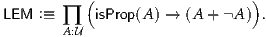 | (3.4.1) |
Similarly, the law of double negation is
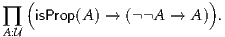 | (3.4.2) |
The two are also easily seen to be equivalent to each other—see Exercise 3.18—so from now on we will generally speak only of LEM.
This formulation of LEM avoids the “paradoxes” of Theorem 3.2.2 and Corollary 3.2.7, since 2 is not a mere proposition. In order to distinguish it from the more general propositions-as-types formulation, we rename the latter:
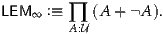 |
For emphasis, the proper version (3.4.1) may be denoted LEM-1; see also Exercise 7.7. Although LEM is not a consequence of the basic type theory described in Chapter 1, it may be consistently assumed as an axiom (unlike its ∞-counterpart). For instance, we will assume it in §10.4.
However, it can be surprising how far we can get without using LEM. Quite often, a simple reformulation of a definition or theorem enables us to avoid invoking excluded middle. While this takes a little getting used to sometimes, it is often worth the hassle, resulting in more elegant and more general proofs. We discussed some of the benefits of this in the introduction.
For instance, in classical mathematics, double negations are frequently used unnecessarily. A very simple example is the common assumption that a set A is “nonempty”, which literally means it is not the case that A contains no elements. Almost always what is really meant is the positive assertion that A does contain at least one element, and by removing the double negation we make the statement less dependent on LEM. Recall that we say that a type A is inhabited when we assert A itself as a proposition (i.e. we construct an element of A, usually unnamed). Thus, often when translating a classical proof into constructive logic, we replace the word “nonempty” by “inhabited” (although sometimes we must replace it instead by “merely inhabited”; see §3.7).
Similarly, it is not uncommon in classical mathematics to find unnecessary proofs by contradiction. Of course, the classical form of proof by contradiction proceeds by way of the law of double negation: we assume ¬A and derive a contradiction, thereby deducing ¬¬A, and thus by double negation we obtain A. However, often the derivation of a contradiction from ¬A can be rephrased slightly so as to yield a direct proof of A, avoiding the need for LEM.
It is also important to note that if the goal is to prove a negation, then “proof by contradiction” does not involve LEM. In fact, since ¬A is by definition the type A →0, by definition to prove ¬A is to prove a contradiction (0) under the assumption of A. Similarly, the law of double negation does hold for negated propositions: ¬¬¬A →¬A. With practice, one learns to distinguish more carefully between negated and non-negated propositions and to notice when LEM is being used and when it is not.
Thus, contrary to how it may appear on the surface, doing mathematics “constructively” does not usually involve giving up important theorems, but rather finding the best way to state the definitions so as to make the important theorems constructively provable. That is, we may freely use the LEM when first investigating a subject, but once that subject is better understood, we can hope to refine its definitions and proofs so as to avoid that axiom. This sort of observation is even more pronounced in homotopy type theory, where the powerful tools of univalence and higher inductive types allow us to constructively attack many problems that traditionally would require classical reasoning. We will see several examples of this in Part II.
It is also worth mentioning that even in constructive mathematics, the law of excluded middle can hold for some propositions. The name traditionally given to such propositions is decidable.
Thus, LEM is exactly the statement that all mere propositions are decidable, and hence so are all families of mere propositions. In particular, LEM implies that all sets (in the sense of §3.1) have decidable equality. Having decidable equality in this sense is very strong; see Theorem 7.2.5.
As another example of the usefulness of mere propositions, we discuss
subsets (and more generally subtypes). Suppose P : A → is a type family,
with each type P(x) regarded as a proposition. Then P itself is a predicate on A,
or a property of elements of A.
In set theory, whenever we have a predicate P on a set A, we may form the
subset  P(x)}. As mentioned briefly in §1.11, the obvious analogue in
type theory is the Σ-type ∑(x:A) P(x). An inhabitant of ∑(x:A) P(x) is, of
course, a pair (x, p) where x : A and p is a proof of P(x). However, for general
P, an element a : A might give rise to more than one distinct element of
∑
(x:A) P(x), if the proposition P(a) has more than one distinct proof. This is
counter to the usual intuition of a subset. But if P is a mere proposition, then
this cannot happen.
P(x)}. As mentioned briefly in §1.11, the obvious analogue in
type theory is the Σ-type ∑(x:A) P(x). An inhabitant of ∑(x:A) P(x) is, of
course, a pair (x, p) where x : A and p is a proof of P(x). However, for general
P, an element a : A might give rise to more than one distinct element of
∑
(x:A) P(x), if the proposition P(a) has more than one distinct proof. This is
counter to the usual intuition of a subset. But if P is a mere proposition, then
this cannot happen.
Lemma 3.5.1. Suppose P : A →is a type family such that P(x) is a mere
proposition for all x : A. If u, v : ∑(x:A) P(x) are such that pr1(u) = pr1(v),
then u = v.
Proof. Suppose p : pr1(u) = pr1(v). By Theorem 2.7.2, to show u = v
it suffices to show p* = pr2(v). But p*
 and pr2(v) are
both elements of P(pr1(v)), which is a mere proposition; hence they are
equal. __
and pr2(v) are
both elements of P(pr1(v)), which is a mere proposition; hence they are
equal. __
For instance, recall that in §2.4 we defined
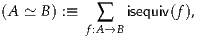
where each type isequiv(f) was supposed to be a mere proposition. It follows that if two equivalences have equal underlying functions, then they are equal as equivalences.
Henceforth, if P : A → is a family of mere propositions (i.e. each P(x) is
a mere proposition), we may write
 | (3.5.2) |
as an alternative notation for ∑(x:A) P(x). (There is no technical reason not to use this notation for arbitrary P as well, but such usage could be confusing due to unintended connotations.) If A is a set, we call (3.5.2) a subset of A; for general A we might call it a subtype. We may also refer to P itself as a subset or subtype of A; this is actually more correct, since the type (3.5.2) in isolation doesn’t remember its relationship to A.
Given such a P and a : A, we may write a ∈ P or a ∈ P(x)}
to refer to the mere proposition P(a). If it holds, we may say that a
is a member of P. Similarly, if
P(x)}
to refer to the mere proposition P(a). If it holds, we may say that a
is a member of P. Similarly, if  Q(x)} is another subset of A,
then we say that P is contained in Q, and write P ⊆ Q, if we have
∏
(x:A) (P(x) → Q(x)).
Q(x)} is another subset of A,
then we say that P is contained in Q, and write P ⊆ Q, if we have
∏
(x:A) (P(x) → Q(x)).
As further examples of subtypes, we may define the “subuniverses” of sets
and of mere propositions in a universe :
| Set | :≡ isSet(A)}, isSet(A)}, | ||
| Prop | :≡ isProp(A)}. isProp(A)}. |
is a type A : together with evidence s : isSet(A), and
similarly for Prop . Lemma 3.5.1 implies that (A, s) =Set (B, t) is
equivalent to A = B (and hence to A ≃ B). Thus, we will frequently abuse
notation and write simply A : Set instead of (A, s) : Set . We may
also drop the subscript if there is no need to specify the universe in
question.
(B, t) is
equivalent to A = B (and hence to A ≃ B). Thus, we will frequently abuse
notation and write simply A : Set instead of (A, s) : Set . We may
also drop the subscript if there is no need to specify the universe in
question.
Recall that for any two universes i and i+1, if A : i then also A : i+1.
Thus, for any (A, s) : Seti we also have (A, s) : Seti+1, and similarly for
Propi, giving natural maps
| Seti | →Seti+1, | (3.5.3) |
| Propi | →Propi+1. | (3.5.4) |
We refer to this axiom as propositional resizing, since it means that any
mere proposition in the universe i+1 can be “resized” to an equivalent one in
the smaller universe i. It follows automatically if i+1 satisfies LEM (see
Exercise 3.10). We will not assume this axiom in general, although in some
places we will use it as an explicit hypothesis. It is a form of impredicativity for
mere propositions, and by avoiding its use, the type theory is said to remain
predicative.
In practice, what we want most frequently is a slightly different statement:
that a universe under consideration contains a type which “classifies all
mere propositions”. In other words, we want a type Ω : together with an
Ω-indexed family of mere propositions, which contains every mere
proposition up to equivalence. This statement follows from propositional
resizing as stated above if is not the smallest universe 0, since then we can
define Ω :≡Prop0.
One use for impredicativity is to define power sets. It is natural to
define the power set of a set A to be A →Prop ; but in the absence of
impredicativity, this definition depends (even up to equivalence) on the choice
of the universe . But with propositional resizing, we can define the power
set to be
which is then independent of . See also §10.1.4.
We mentioned in §1.1 that in contrast to type theory, which has only one basic notion (types), set-theoretic foundations have two basic notions: sets and propositions. Thus, a classical mathematician is accustomed to manipulating these two kinds of objects separately.
It is possible to recover a similar dichotomy in type theory, with the role of the set-theoretic propositions being played by the types (and type families) that are mere propositions. In many cases, the logical connectives and quantifiers can be represented in this logic by simply restricting the corresponding type-former to the mere propositions. Of course, this requires knowing that the type-former in question preserves mere propositions.
Example 3.6.1. If A and B are mere propositions, so is A × B. This is easy to show using the characterization of paths in products, just like Example 3.1.5 but simpler. Thus, the connective “and” preserves mere propositions.
Example 3.6.2. If A is any type and B : A → is such that for all
x : A, the type B(x) is a mere proposition, then ∏(x:A) B(x) is a mere
proposition. The proof is just like Example 3.1.6 but simpler: given
f, g : ∏(x:A) B(x), for any x : A we have f(x) = g(x) since B(x) is a mere
proposition. But then by function extensionality, we have f = g.
In particular, if B is a mere proposition, then so is A → B regardless of what A is. In even more particular, since 0 is a mere proposition, so is ¬A ≡ (A →0). Thus, the connectives “implies” and “not” preserve mere propositions, as does the quantifier “for all”.
On the other hand, some type formers do not preserve mere propositions. Even if A and B are mere propositions, A + B will not in general be. For instance, 1 is a mere proposition, but 2 = 1 + 1 is not. Logically speaking, A + B is a “purely constructive” sort of “or”: a witness of it contains the additional information of which disjunct is true. Sometimes this is very useful, but if we want a more classical sort of “or” that preserves mere propositions, we need a way to “truncate” this type into a mere proposition by forgetting this additional information.
The same issue arises with the Σ-type ∑(x:A) P(x). This is a purely constructive interpretation of “there exists an x : A such that P(x)” which remembers the witness x, and hence is not generally a mere proposition even if each type P(x) is. (Recall that we observed in §3.5 that ∑ (x:A) P(x) can also be regarded as “the subset of those x : A such that P(x)”.)
The propositional truncation, also called the (-1)-truncation, bracket type, or squash type, is an additional type former which “squashes” or “truncates” a type down to a mere proposition, forgetting all information contained in inhabitants of that type other than their existence.
More precisely, for any type A, there is a type  . It has two
constructors:
. It has two
constructors:
 :
:  .
.
 , we have x = y.
The first constructor means that if A is inhabited, so is  . The second ensures
that
. The second ensures
that  is a mere proposition; usually we leave the witness of this fact
nameless.
is a mere proposition; usually we leave the witness of this fact
nameless.
The recursion principle of  says that:
 → B such that g(
 ) ≡ f(a) for all a : A.
In other words, any mere proposition which follows from (the inhabitedness
of) A already follows from  . Thus,
  , as a mere proposition,
contains no more information than the inhabitedness of A. (There is also
an induction principle for
, as a mere proposition,
contains no more information than the inhabitedness of A. (There is also
an induction principle for  , but it is not especially useful; see
Exercise 3.17.)
, but it is not especially useful; see
Exercise 3.17.)
In Exercises 3.14 and 3.15 and §6.9 we will describe some ways to
construct  in terms of more general things. For now, we simply assume it
as an additional rule alongside those of Chapter 1.
in terms of more general things. For now, we simply assume it
as an additional rule alongside those of Chapter 1.
With the propositional truncation, we can extend the “logic of mere
propositions” to cover disjunction and the existential quantifier. Specifically,
 is a mere propositional version of “A or B”, which does not
“remember” the information of which disjunct is true.
is a mere propositional version of “A or B”, which does not
“remember” the information of which disjunct is true.
The recursion principle of truncation implies that we can still do a
case analysis on  when attempting to prove a mere proposition.
That is, suppose we have an assumption u :
when attempting to prove a mere proposition.
That is, suppose we have an assumption u :  and we are
trying to prove a mere proposition Q. In other words, we are trying to
define an element of
and we are
trying to prove a mere proposition Q. In other words, we are trying to
define an element of  → Q. Since Q is a mere proposition,
by the recursion principle for propositional truncation, it suffices to
construct a function A + B → Q. But now we can use case analysis on
A + B.
→ Q. Since Q is a mere proposition,
by the recursion principle for propositional truncation, it suffices to
construct a function A + B → Q. But now we can use case analysis on
A + B.
Similarly, for a type family P : A →, we can consider  ,
which is a mere propositional version of “there exists an x : A such that P(x)”.
As for disjunction, by combining the induction principles of truncation and
Σ-types, if we have an assumption of type
,
which is a mere propositional version of “there exists an x : A such that P(x)”.
As for disjunction, by combining the induction principles of truncation and
Σ-types, if we have an assumption of type  , we may introduce
new assumptions x : A and y : P(x) when attempting to prove a mere proposition.
In other words, if we know that there exists some x : A such that P(x), but we
don’t have a particular such x in hand, then we are free to make use
of such an x as long as we aren’t trying to construct anything which
might depend on the particular value of x. Requiring the codomain
to be a mere proposition expresses this independence of the result
on the witness, since all possible inhabitants of such a type must be
equal.
, we may introduce
new assumptions x : A and y : P(x) when attempting to prove a mere proposition.
In other words, if we know that there exists some x : A such that P(x), but we
don’t have a particular such x in hand, then we are free to make use
of such an x as long as we aren’t trying to construct anything which
might depend on the particular value of x. Requiring the codomain
to be a mere proposition expresses this independence of the result
on the witness, since all possible inhabitants of such a type must be
equal.
For the purposes of set-level mathematics in Chapters 10 and 11, where we deal mostly with sets and mere propositions, it is convenient to use the traditional logical notations to refer only to “propositionally truncated logic”.
Definition 3.7.1. We define traditional logical notation using truncation as follows, where P and Q denote mere propositions (or families thereof):
| ⊤ | :≡ 1 | ||
| ⊥ | :≡ 0 | ||
| P ∧Q | :≡ P ×Q | ||
| P ⇒ Q | :≡ P → Q | ||
| P ⇔ Q | :≡ P = Q | ||
| ¬P | :≡ P →0 | ||
| P ∨Q | :≡  | ||
| ∀(x : A).P(x) | :≡ ∏ x:AP(x) | ||
| ∃(x : A).P(x) | :≡  ∑
x:AP(x) ∑
x:AP(x) |
The notations ∧ and ∨ are also used in homotopy theory for the smash product and the wedge of pointed spaces, which we will introduce in Chapter 6. This technically creates a potential for conflict, but no confusion will generally arise.
Similarly, when discussing subsets as in §3.5, we may use the traditional notation for intersections, unions, and complements:
 P(x)}∩ P(x)}∩ Q(x)} Q(x)} | :≡ P(x) ∧Q(x)}, P(x) ∧Q(x)}, | ||
 P(x)}∪ P(x)}∪ Q(x)} Q(x)} | :≡ P(x) ∨Q(x)}, P(x) ∨Q(x)}, | ||
A\ P(x)} P(x)} | :≡ ¬P(x)}. ¬P(x)}. |
We can now properly formulate the axiom of choice in homotopy type theory. Assume a type X and type families
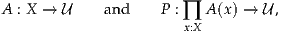 |
and moreover that
The axiom of choice AC asserts that under these assumptions,
 | (3.8.1) |
Of course, this is a direct translation of (3.2.1) where we read “there exists
x : A such that B(x)” as  , so we could have written the
statement in the familiar logical notation as
, so we could have written the
statement in the familiar logical notation as
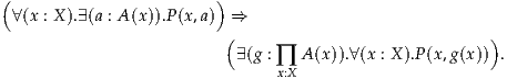
In fact, because of Theorem 2.15.7, this axiom can also be expressed in a simpler form.
Lemma 3.8.2. The axiom of choice (3.8.1) is equivalent to the statement that for
any set X and any Y : X →such that each Y(x) is a set, we have
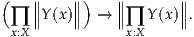 | (3.8.3) |
This corresponds to a well-known equivalent form of the classical axiom of choice, namely “the cartesian product of a family of nonempty sets is nonempty”.
Proof. By Theorem 2.15.7, the codomain of (3.8.1) is equivalent to
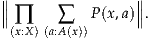
Thus, (3.8.1) is equivalent to the instance of (3.8.3) where
 |
Conversely, (3.8.3) is equivalent to the instance of (3.8.1) where A(x) :≡ Y(x) and P(x, a) :≡1. Thus, the two are logically equivalent. Since both are mere propositions, by Lemma 3.3.3 they are equivalent types. __
As with LEM, the equivalent forms (3.8.1) and (3.8.3) are not a consequence of our basic type theory, but they may consistently be assumed as axioms.
Remark 3.8.4. It is easy to show that the right side of (3.8.3) always implies the left. Since both are mere propositions, by Lemma 3.3.3 the axiom of choice is also equivalent to asking for an equivalence
This illustrates a common pitfall: although dependent function types
preserve mere propositions (Example 3.6.2), they do not commute with
truncation:  is not generally equivalent to ∏(x:A)
  .
The axiom of choice, if we assume it, says that this is true for sets; as we
will see below, it fails in general.
.
The axiom of choice, if we assume it, says that this is true for sets; as we
will see below, it fails in general.
The restriction in the axiom of choice to types that are sets can be relaxed to a certain extent. For instance, we may allow A and P in (3.8.1), or Y in (3.8.3), to be arbitrary type families; this results in a seemingly stronger statement that is equally consistent. We may also replace the propositional truncation by the more general n-truncations to be considered in Chapter 7, obtaining a spectrum of axioms ACn interpolating between (3.8.1), which we call simply AC (or AC-1 for emphasis), and Theorem 2.15.7, which we shall call AC∞. See also Exercises 7.8 and 7.10. However, observe that we cannot relax the requirement that X be a set.
Lemma 3.8.5. There exists a type X and a family Y : X →such that each
Y(x) is a set, but such that (3.8.3) is false.
Proof. Define X :≡ ∑(A:)  , and let x0 :≡ (2,
  ) : X.
Then by the identification of paths in Σ-types, the fact that
) : X.
Then by the identification of paths in Σ-types, the fact that  is
a mere proposition, and univalence, for any (A, p), (B, q) : X we have
((A, p) =X (B, q)) ≃ (A ≃ B). In particular, (x0 =X x0) ≃ (2 ≃2), so as
in Example 3.1.9, X is not a set.
is
a mere proposition, and univalence, for any (A, p), (B, q) : X we have
((A, p) =X (B, q)) ≃ (A ≃ B). In particular, (x0 =X x0) ≃ (2 ≃2), so as
in Example 3.1.9, X is not a set.
On the other hand, if (A, p) : X, then A is a set; this follows by
induction on truncation for p :  and the fact that 2 is a set. Since
A ≃ B is a set whenever A and B are, it follows that x1 =X x2 is a set for
any x1, x2 : X, i.e. X is a 1-type. In particular, if we define Y : X → by
Y(x) :≡ (x0 = x), then each Y(x) is a set.
and the fact that 2 is a set. Since
A ≃ B is a set whenever A and B are, it follows that x1 =X x2 is a set for
any x1, x2 : X, i.e. X is a 1-type. In particular, if we define Y : X → by
Y(x) :≡ (x0 = x), then each Y(x) is a set.
Now by definition, for any (A, p) : X we have  , and hence
 . Thus, we have ∏(x:X)
  . If (3.8.3) held for this X
and Y, then we would also have
. If (3.8.3) held for this X
and Y, then we would also have  . Since we are trying to
derive a contradiction (0), which is a mere proposition, we may assume
∏
(x:X) Y(x), i.e. that ∏(x:X) (x0 = x). But this implies X is a mere
proposition, and hence a set, which is a contradiction. __
. Since we are trying to
derive a contradiction (0), which is a mere proposition, we may assume
∏
(x:X) Y(x), i.e. that ∏(x:X) (x0 = x). But this implies X is a mere
proposition, and hence a set, which is a contradiction. __
The following observation is trivial, but very useful.
Proof. Of course, we have P → by definition. And since P is a mere
proposition, the universal property of
by definition. And since P is a mere
proposition, the universal property of  applied to idP : P → P yields
 → P. These functions are quasi-inverses by Lemma 3.3.3. __
Among its important consequences is the following.
Corollary 3.9.2 (The principle of unique choice). Suppose a type family
P : A →such that
 .
.Then we have ∏(x:A) P(x).
Proof. Immediate from the two assumptions and the previous lemma. __
The corollary also encapsulates a very useful technique of reasoning.
Namely, suppose we know that  , and we want to use this to construct an
element of some other type B. We would like to use an element of A in our
construction of an element of B, but this is allowed only if B is a mere
proposition, so that we can apply the induction principle for the propositional
truncation
, and we want to use this to construct an
element of some other type B. We would like to use an element of A in our
construction of an element of B, but this is allowed only if B is a mere
proposition, so that we can apply the induction principle for the propositional
truncation  ; the most we could hope to do in general is to show
  .
Instead, we can extend B with additional data which characterizes uniquely
the object we wish to construct. Specifically, we define a predicate Q : B →
such that ∑(x:B) Q(x) is a mere proposition. Then from an element of A we
construct an element b : B such that Q(b), hence from
.
Instead, we can extend B with additional data which characterizes uniquely
the object we wish to construct. Specifically, we define a predicate Q : B →
such that ∑(x:B) Q(x) is a mere proposition. Then from an element of A we
construct an element b : B such that Q(b), hence from  we can construct
 , and because
  is equivalent to ∑(x:B) Q(x) an
element of B may be projected from it. An example can be found in
Exercise 3.19.
is equivalent to ∑(x:B) Q(x) an
element of B may be projected from it. An example can be found in
Exercise 3.19.
A similar issue arises in set-theoretic mathematics, although it manifests
slightly differently. If we are trying to define a function f : A → B, and
depending on an element a : A we are able to prove mere existence of some
b : B, we are not done yet because we need to actually pinpoint an element
of B, not just prove its existence. One option is of course to refine the
argument to unique existence of b : B, as we did in type theory. But in set
theory the problem can often be avoided more simply by an application of the
axiom of choice, which picks the required elements for us. In homotopy
type theory, however, quite apart from any desire to avoid choice, the
available forms of choice are simply less applicable, since they require that
the domain of choice be a set. Thus, if A is not a set (such as perhaps
a universe ), there is no consistent form of choice that will allow
us to simply pick an element of B for each a : A to use in defining
f(a).
At first glance, it may seem that the truncated versions of + and Σ are actually closer to the informal mathematical meaning of “or” and “there exists” than the untruncated ones. Certainly, they are closer to the precise meaning of “or” and “there exists” in the first-order logic which underlies formal set theory, since the latter makes no attempt to remember any witnesses to the truth of propositions. However, it may come as a surprise to realize that the practice of informal mathematics is often more accurately described by the untruncated forms.
For example, consider a statement like “every prime number is either 2 or odd”. The working mathematician feels no compunction about using this fact not only to prove theorems about prime numbers, but also to perform constructions on prime numbers, perhaps doing one thing in the case of 2 and another in the case of an odd prime. The end result of the construction is not merely the truth of some statement, but a piece of data which may depend on the parity of the prime number. Thus, from a type-theoretic perspective, such a construction is naturally phrased using the induction principle for the coproduct type “(p = 2) + (p is odd)”, not its propositional truncation.
Admittedly, this is not an ideal example, since “p = 2” and “p is odd” are mutually exclusive, so that (p = 2) + (p is odd) is in fact already a mere proposition and hence equivalent to its truncation (see Exercise 3.7). More compelling examples come from the existential quantifier. It is not uncommon to prove a theorem of the form “there exists an x such that …” and then refer later on to “the x constructed in Theorem Y” (note the definite article). Moreover, when deriving further properties of this x, one may use phrases such as “by the construction of x in the proof of Theorem Y”.
A very common example is “A is isomorphic to B”, which strictly speaking means only that there exists some isomorphism between A and B. But almost invariably, when proving such a statement, one exhibits a specific isomorphism or proves that some previously known map is an isomorphism, and it often matters later on what particular isomorphism was given.
Set-theoretically trained mathematicians often feel a twinge of guilt at such “abuses of language”. We may attempt to apologize for them, expunge them from final drafts, or weasel out of them with vague words like “canonical”. The problem is exacerbated by the fact that in formalized set theory, there is technically no way to “construct” objects at all — we can only prove that an object with certain properties exists. Untruncated logic in type theory thus captures some common practices of informal mathematics that the set theoretic reconstruction obscures. (This is similar to how the univalence axiom validates the common, but formally unjustified, practice of identifying isomorphic objects.)
On the other hand, sometimes truncated logic is essential. We have seen this in the statements of LEM and AC; some other examples will appear later on in the book. Thus, we are faced with the problem: when writing informal type theory, what should we mean by the words “or” and “there exists” (along with common synonyms such as “there is” and “we have”)?
A universal consensus may not be possible. Perhaps depending on the sort
of mathematics being done, one convention or the other may be more useful
— or, perhaps, the choice of convention may be irrelevant. In this case, a
remark at the beginning of a mathematical paper may suffice to inform the
reader of the linguistic conventions in use therein. However, even after one
overall convention is chosen, the other sort of logic will usually arise at least
occasionally, so we need a way to refer to it. More generally, one may
consider replacing the propositional truncation with another operation on
types that behaves similarly, such as the double negation operation
A ¬¬A, or the n-truncations to be considered in Chapter 7. As an
experiment in exposition, in what follows we will occasionally use
adverbs to denote the application of such “modalities” as propositional
truncation.
¬¬A, or the n-truncations to be considered in Chapter 7. As an
experiment in exposition, in what follows we will occasionally use
adverbs to denote the application of such “modalities” as propositional
truncation.
For instance, if untruncated logic is the default convention, we may use the adverb merely to denote propositional truncation. Thus the phrase
“there merely exists an x : A such that P(x)”
indicates the type  . Similarly, we will say that a type A is merely
inhabited to mean that its propositional truncation
. Similarly, we will say that a type A is merely
inhabited to mean that its propositional truncation  is inhabited (i.e. that
we have an unnamed element of it). Note that this is a definition of the adverb
“merely” as it is to be used in our informal mathematical English, in the same
way that we define nouns like “group” and “ring”, and adjectives like
“regular” and “normal”, to have precise mathematical meanings. We are not
claiming that the dictionary definition of “merely” refers to propositional
truncation; the choice of word is meant only to remind the mathematician
reader that a mere proposition contains “merely” the information of a truth
value and nothing more.
is inhabited (i.e. that
we have an unnamed element of it). Note that this is a definition of the adverb
“merely” as it is to be used in our informal mathematical English, in the same
way that we define nouns like “group” and “ring”, and adjectives like
“regular” and “normal”, to have precise mathematical meanings. We are not
claiming that the dictionary definition of “merely” refers to propositional
truncation; the choice of word is meant only to remind the mathematician
reader that a mere proposition contains “merely” the information of a truth
value and nothing more.
On the other hand, if truncated logic is the current default convention, we may use an adverb such as purely or constructively to indicate its absence, so that
“there purely exists an x : A such that P(x)”
would denote the type ∑(x:A) P(x). We may also use “purely” or “actually” just to emphasize the absence of truncation, even when that is the default convention.
In this book we will continue using untruncated logic as the default convention, for a number of reasons.
In Lemma 3.3.2 we observed that a mere proposition which is inhabited must be equivalent to 1, and it is not hard to see that the converse also holds. A type with this property is called contractible. Another equivalent definition of contractibility, which is also sometimes convenient, is the following.
Definition 3.11.1. A type A is contractible, or a singleton, if there is a : A, called the center of contraction, such that a = x for all x : A. We denote the specified path a = x by contrx.
In other words, the type isContr(A) is defined to be
Note that under the usual propositions-as-types reading, we can pronounce isContr(A) as “A contains exactly one element”, or more precisely “A contains an element, and every element of A is equal to that element”.
Remark 3.11.2. We can also pronounce isContr(A) more topologically as
“there is a point a : A such that for all x : A there exists a path from
a to x”. Note that to a classical ear, this sounds like a definition of
connectedness rather than contractibility. The point is that the meaning
of “there exists” in this sentence is a continuous/natural one. A more
correct way to express connectedness would be ∑(a:A) ∏(x:A)  ;
see Lemma 7.5.11.
;
see Lemma 7.5.11.
Lemma 3.11.3. For a type A, the following are logically equivalent.
Proof. If A is contractible, then it certainly has a point a : A (the center of contraction), while for any x, y : A we have x = a = y; thus A is a mere proposition. Conversely, if we have a : A and A is a mere proposition, then for any x : A we have x = a; thus A is contractible. And we showed (ii)⇒(iii) in Lemma 3.3.2, while the converse follows since 1 easily has property (ii). __
Proof. Suppose given c, c′ : isContr(A). We may assume c ≡ (a, p) and
c′≡ (a′, p′) for a, a′ : A and p : ∏(x:A) (a = x) and p′ : ∏(x:A) (a′ = x).
By the characterization of paths in Σ-types, to show c = c′ it suffices to
exhibit q : a = a′ such that q* = p′. We choose q :≡ p(a′). Now since
A is contractible (by c or c′), by Lemma 3.11.3 it is a mere proposition.
Hence, by Lemma 3.3.4 and Example 3.6.2, so is ∏(x:A) (a′ = x); thus
q*
= p′. We choose q :≡ p(a′). Now since
A is contractible (by c or c′), by Lemma 3.11.3 it is a mere proposition.
Hence, by Lemma 3.3.4 and Example 3.6.2, so is ∏(x:A) (a′ = x); thus
q* = p′ is automatic. __
Proof. By Lemma 3.11.4 and Lemma 3.11.3(ii). __
Like mere propositions, contractible types are preserved by many type constructors. For instance, we have:
Lemma 3.11.6. If P : A → is a type family such that each P(a) is
contractible, then ∏(x:A) P(x) is contractible.
Proof. By Example 3.6.2, ∏(x:A) P(x) is a mere proposition since each P(x) is. But it also has an element, namely the function sending each x : A to the center of contraction of P(x). Thus by Lemma 3.11.3(ii), ∏ (x:A) P(x) is contractible. __
(In fact, the statement of Lemma 3.11.6 is equivalent to the function extensionality axiom. See §4.9.)
Of course, if A is equivalent to B and A is contractible, then so is B. More generally, it suffices for B to be a retract of A. By definition, a retraction is a function r : A → B such that there exists a function s : B → A, called its section, and a homotopy ϵ : ∏(y:B) (r(s(y)) = y); then we say that B is a retract of A.
Proof. Let a0 : A be the center of contraction. We claim that b0 :≡ r(a0) : B is a center of contraction for B. Let b : B; we need a path b = b0. But we have ϵb : r(s(b)) = b and contrs(b) : s(b) = a0, so by composition

Contractible types may not seem very interesting, since they are all equivalent to 1. One reason the notion is useful is that sometimes a collection of individually nontrivial data will collectively form a contractible type. An important example is the space of paths with one free endpoint. As we will see in §5.8, this fact essentially encapsulates the based path induction principle for identity types.
Proof. We choose as center the point (a, refla). Now suppose (x, p) :
∑
(x:A) (a = x); we must show (a, refla) = (x, p). By the characterization
of paths in Σ-types, it suffices to exhibit q : a = x such that q* = p.
But we can take q :≡ p, in which case q*
= p.
But we can take q :≡ p, in which case q* = p follows from the
characterization of transport in path types. __
= p follows from the
characterization of transport in path types. __
When this happens, it can allow us to simplify a complicated construction up to equivalence, using the informal principle that contractible data can be freely ignored. This principle consists of many lemmas, most of which we leave to the reader; the following is an example.
Proof. In the situation of (i), we show that pr1 : ∑(x:A) P(x) → A is an equivalence. For quasi-inverse we define g(x) :≡ (x, cx) where cx is the center of P(x). The composite pr1 ∘g is obviously idA, whereas the opposite composite is homotopic to the identity by using the contractions of each P(x).
We leave the proof of (ii) to the reader (see Exercise 3.20). __
Another reason contractible types are interesting is that they extend the ladder of n-types mentioned in §3.1 downwards one more step.
Lemma 3.11.10. A type A is a mere proposition if and only if for all x, y : A, the type x =A yis contractible.
Proof. For “if”, we simply observe that any contractible type is inhabited. For “only if”, we observed in §3.3 that every mere proposition is a set, so that each type x =A y is a mere proposition. But it is also inhabited (since A is a mere proposition), and hence by Lemma 3.11.3(ii) it is contractible. __
Thus, contractible types may also be called (-2)-types. They are the bottom rung of the ladder of n-types, and will be the base case of the recursive definition of n-types in Chapter 7.
The fact that it is possible to define sets, mere propositions, and contractible types in type theory, with all higher homotopies automatically taken care of as in §§3.1, 3.3 and 3.11, was first observed by Voevodsky. In fact, he defined the entire hierarchy of n-types by induction, as we will do in Chapter 7.
Theorem 3.2.2 and Corollary 3.2.7 rely in essence on a classical theorem of Hedberg, which we will prove in §7.2. The implication that the propositions-as-types form of LEM contradicts univalence was observed by Martín Escardó on the Agda mailing list. The proof we have given of Theorem 3.2.2 is due to Thierry Coquand.
The propositional truncation was introduced in the extensional type theory of NuPRL in 1983 by Constable [Con85] as an application of “subset” and “quotient” types. What is here called the “propositional truncation” was called “squashing” in the NuPRL type theory [CAB+86]. Rules characterizing the propositional truncation directly, still in extensional type theory, were given in [AB04]. The intensional version in homotopy type theory was constructed by Voevodsky using an impredicative quantification, and later by Lumsdaine using higher inductive types (see §6.9).
Voevodsky [Voe12] has proposed resizing rules of the kind considered in §3.5. These are clearly related to the notorious axiom of reducibility proposed by Russell in his and Whitehead’s Principia Mathematica [WR27].
The adverb “purely” as used to refer to untruncated logic is a reference to the use of monadic modalities to model effects in programming languages; see §7.7 and the Notes to Chapter 7.
There are many different ways in which logic can be treated relative to type theory. For instance, in addition to the plain propositions-as-types logic described in §1.11, and the alternative which uses mere propositions only as described in §3.6, one may introduce a separate “sort” of propositions, which behave somewhat like types but are not identified with them. This is the approach taken in logic enriched type theory [AG02] and in some presentations of the internal languages of toposes and related categories (e.g. [Jac99, Joh02]), as well as in the proof assistant Coq. Such an approach is more general, but less powerful. For instance, the principle of unique choice (§3.9) fails in the category of so-called setoids in Coq [Spi11], in logic enriched type theory [AG02], and in minimal type theory [MS05]. Thus, the univalence axiom makes our type theory behave more like the internal logic of a topos; see also Chapter 10.
Martin-Löf [ML06] provides a discussion on the history of axioms of choice. Of course, constructive and intuitionistic mathematics has a long and complicated history, which we will not delve into here; see for instance [TvD88a, TvD88b].
Exercise 3.3. Prove that if A is a set and B : A → is a type family such
that B(x) is a set for all x : A, then ∑(x:A) B(x) is a set.
Exercise 3.6. Show that if A is a mere proposition, then so is A + (¬A). Thus, there is no need to insert a propositional truncation in (3.4.1).
Exercise 3.7. More generally, show that if A and B are mere propositions and ¬(A×B), then A + B is also a mere proposition.
Exercise 3.8. Assuming that some type isequiv(f)
satisfies conditions (i)–(iii) of §2.4, show that the type  satisfies
the same conditions and is equivalent to isequiv(f).
satisfies
the same conditions and is equivalent to isequiv(f).
Exercise 3.10. Show that if i+1 satisfies LEM, then the canonical
inclusion Propi →Propi+1 is an equivalence.
Exercise 3.11. Show that it is not the case that for all A : we have
 → A. (However, there can be particular types for which
  → A.
Exercise 3.8 implies that qinv(f) is such.)
→ A.
Exercise 3.8 implies that qinv(f) is such.)
Exercise 3.12. Show that if LEM holds, then for all A : we have
 (
( → A)
→ A) . (This property is a very simple form of the axiom of
choice, which can fail in the absence of LEM; see [KECA13].)
. (This property is a very simple form of the axiom of
choice, which can fail in the absence of LEM; see [KECA13].)
Exercise 3.13. We showed in Corollary 3.2.7 that the following naive form of LEM is inconsistent with univalence:
In the absence of univalence, this axiom is consistent. However, show that it implies the axiom of choice (3.8.1).
Exercise 3.14. Show that assuming LEM, the double negation ¬¬A has
the same universal property as the propositional truncation  , and is
therefore equivalent to it. Thus, under LEM, the propositional truncation
can be defined rather than taken as a separate type former.
, and is
therefore equivalent to it. Thus, under LEM, the propositional truncation
can be defined rather than taken as a separate type former.
Exercise 3.15. Show that if we assume propositional resizing as in §3.5, then the type
has the same universal property as  . Thus, we can also define the
propositional truncation in this case.
. Thus, we can also define the
propositional truncation in this case.
Exercise 3.16. Assuming LEM, show that double negation commutes with universal quantification of mere propositions over sets. That is, show that if X is a set and each Y(x) is a mere proposition, then LEM implies
 | (3.11.11) |
Observe that if we assume instead that each Y(x) is a set, then (3.11.11) becomes equivalent to the axiom of choice (3.8.3).
Exercise 3.17. Show that the rules for the propositional truncation given
in §3.7 are sufficient to imply the following induction principle: for any
type family B :  → such that each B(x) is a mere proposition, if
for every a : A we have B(
→ such that each B(x) is a mere proposition, if
for every a : A we have B( ), then for every x :
  we have B(x).
Exercise 3.18. Show that the law of excluded middle (3.4.1) and the law of double negation (3.4.2) are logically equivalent.
Exercise 3.20. Prove Lemma 3.11.9(ii): if A is contractible with center a, then ∑(x:A) P(x) is equivalent to P(a).
Exercise 3.22. As in classical set theory, the finite version of the axiom of choice is a theorem. Prove that the axiom of choice (3.8.1) holds when X is a finite type Fin(n) (as defined in Exercise 1.9).
We now study in more detail the notion of equivalence of types that was introduced briefly in §2.4. Specifically, we will give several different ways to define a type isequiv(f) having the properties mentioned there. Recall that we wanted isequiv(f) to have the following properties, which we restate here:
Here qinv(f) denotes the type of quasi-inverses to f:
 |
By function extensionality, it follows that qinv(f) is equivalent to the type
 |
We will define three different types having properties (i)–(iii), which we call
We will also show that all these types are equivalent. These names are intentionally somewhat cumbersome, because after we know that they are all equivalent and have properties (i)–(iii), we will revert to saying simply “equivalence” without needing to specify which particular definition we choose. But for purposes of the comparisons in this chapter, we need different names for each definition.
Before we examine the different notions of equivalence, however, we give a little more explanation of why a different concept than quasi-invertibility is needed.
We have said that qinv(f) is unsatisfactory because it is not a mere proposition, whereas we would rather that a given function can “be an equivalence” in at most one way. However, we have given no evidence that qinv(f) is not a mere proposition. In this section we exhibit a specific counterexample.
Proof. By assumption, f is an equivalence; that is, we have e : isequiv(f) and so (f, e) : A ≃ B. By univalence, idtoeqv : (A = B) → (A ≃ B) is an equivalence, so we may assume that (f, e) is of the form idtoeqv(p) for some p : A = B. Then by path induction, we may assume p is reflA, in which case idtoeqv(p) is idA. Thus we are reduced to proving qinv(idA) ≃ ( ∏(x:A) (x = x)). Now by definition we have
By function extensionality, this is equivalent to
And by Exercise 2.10, this is equivalent to
However, by Lemma 3.11.8, ∑(g:A→A) (g = idA) is contractible with center idA; therefore by Lemma 3.11.9 this type is equivalent to idA = idA. And by function extensionality, idA = idA is equivalent to ∏ (x:A) x = x. __
We remark that Exercise 4.3 asks for a proof of the above lemma which avoids univalence.
Thus, what we need is some A which admits a nontrivial element of ∏ (x:A) (x = x). Thinking of A as a higher groupoid, an inhabitant of ∏ (x:A) (x = x) is a natural transformation from the identity functor of A to itself. Such transformations are said to form the center of a category, since the naturality axiom requires that they commute with all morphisms. Classically, if A is simply a group regarded as a one-object groupoid, then this yields precisely its center in the usual group-theoretic sense. This provides some motivation for the following.
Lemma 4.1.2. Suppose we have a type A with a : A and q : a = a such that
Then there exists f : ∏(x:A) (x = x) with f(a) = q.
Proof. Let g : ∏(x:A)  be as given by (ii). First we observe that
each type x =A y is a set. For since being a set is a mere proposition,
we may apply the induction principle of propositional truncation, and
assume that g(x) =
be as given by (ii). First we observe that
each type x =A y is a set. For since being a set is a mere proposition,
we may apply the induction principle of propositional truncation, and
assume that g(x) =  and g(y) =
  for p : a = x and q : a = y. In this
case, composing with p and q-1 yields an equivalence (x = y) ≃ (a = a).
But (a = a) is a set by (i), so (x = y) is also a set.
for p : a = x and q : a = y. In this
case, composing with p and q-1 yields an equivalence (x = y) ≃ (a = a).
But (a = a) is a set by (i), so (x = y) is also a set.
Now, we would like to define f by assigning to each x the path
g(x)-1 ▪q▪g(x), but this does not work because g(x) does not inhabit
a = x but rather  , and the type (x = x) may not be a mere
proposition, so we cannot use induction on propositional truncation.
Instead we can apply the technique mentioned in §3.9: we characterize
uniquely the object we wish to construct. Let us define, for each x : A,
the type
, and the type (x = x) may not be a mere
proposition, so we cannot use induction on propositional truncation.
Instead we can apply the technique mentioned in §3.9: we characterize
uniquely the object we wish to construct. Let us define, for each x : A,
the type
We claim that B(x) is a mere proposition for each x : A. Since this claim
is itself a mere proposition, we may again apply induction on truncation
and assume that g(x) =  for some p : a = x. Now suppose given
(r, h) and (r′, h′) in B(x); then we have
for some p : a = x. Now suppose given
(r, h) and (r′, h′) in B(x); then we have
It remains to show that h is identified with h′ when transported along this equality, which by transport in identity types and function types (§§2.9 and 2.11), reduces to showing
for any s : a = x. But each side of this is an equality between elements of (x = x), so it follows from our above observation that (x = x) is a set.
Thus, each B(x) is a mere proposition; we claim that ∏(x:A) B(x).
Given x : A, we may now invoke the induction principle of propositional
truncation to assume that g(x) =  for p : a = x. We define
r :≡ p-1 ▪q▪p; to inhabit B(x) it remains to show that for any s : a = x
we have r = s-1 ▪q▪s. Manipulating paths, this reduces to showing that
q▪ (p▪s-1) = (p▪s-1) ▪q. But this is just an instance of (iii). __
for p : a = x. We define
r :≡ p-1 ▪q▪p; to inhabit B(x) it remains to show that for any s : a = x
we have r = s-1 ▪q▪s. Manipulating paths, this reduces to showing that
q▪ (p▪s-1) = (p▪s-1) ▪q. But this is just an instance of (iii). __
Theorem 4.1.3. There exist types A and B and a function f : A → B such that qinv(f) is not a mere proposition.
Proof. It suffices to exhibit a type X such that ∏(x:X) (x = x) is not
a mere proposition. Define X :≡ ∑(A:)  , as in the proof of
Lemma 3.8.5. It will suffice to exhibit an f : ∏(x:X) (x = x) which is
unequal to λx.reflx.
, as in the proof of
Lemma 3.8.5. It will suffice to exhibit an f : ∏(x:X) (x = x) which is
unequal to λx.reflx.
Let a :≡ (2,  ) : X, and let q : a = a be the path corresponding
to the nonidentity equivalence e : 2 ≃ 2 defined by e(02) :≡ 12 and
e(12) :≡ 02. We would like to apply Lemma 4.1.2 to build an f. By
definition of X, equalities in subset types (§3.5), and univalence, we have
(a = a) ≃ (2 ≃2), which is a set, so (i) holds. Similarly, by definition
of X and equalities in subset types we have (ii). Finally, Exercise 2.13
implies that every equivalence 2 ≃2 is equal to either id2 or e, so we can
show (iii) by a four-way case analysis.
) : X, and let q : a = a be the path corresponding
to the nonidentity equivalence e : 2 ≃ 2 defined by e(02) :≡ 12 and
e(12) :≡ 02. We would like to apply Lemma 4.1.2 to build an f. By
definition of X, equalities in subset types (§3.5), and univalence, we have
(a = a) ≃ (2 ≃2), which is a set, so (i) holds. Similarly, by definition
of X and equalities in subset types we have (ii). Finally, Exercise 2.13
implies that every equivalence 2 ≃2 is equal to either id2 or e, so we can
show (iii) by a four-way case analysis.
Thus, we have f : ∏(x:X) (x = x) such that f(a) = q. Since e is not equal to id2, q is not equal to refla, and thus f is not equal to λx.reflx. Therefore, ∏(x:X) (x = x) is not a mere proposition. __
More generally, Lemma 4.1.2 implies that any “Eilenberg–Mac Lane space” K(G, 1), where G is a nontrivial abelian group, will provide a counterexample; see Chapter 8. The type X we used turns out to be equivalent to K(Z2, 1). In Chapter 6 we will see that the circle S1 = K(Z, 1) is another easy-to-describe example.
We now move on to describing better notions of equivalence.
In §4.1 we concluded that qinv(f) is equivalent to ∏(x:A) (x = x) by discarding a contractible type. Roughly, the type qinv(f) contains three data g, η, and ϵ, of which two (g and η) could together be seen to be contractible when f is an equivalence. The problem is that removing these data left one remaining (ϵ). In order to solve this problem, the idea is to add one additional datum which, together with ϵ, forms a contractible type.
Definition 4.2.1. A function f : A → B is a half adjoint equivalence if there are g : B → A and homotopies η : g∘f ~idA and ϵ : f ∘g ~idB such that there exists a homotopy
Thus we have a type ishae(f), defined to be
 |
Note that in the above definition, the coherence condition relating η and ϵ only involves f. We might consider instead an analogous coherence condition involving g:
and a resulting analogous definition ishae′(f).
Fortunately, it turns out each of the conditions implies the other one:
Lemma 4.2.2. For functions f : A → B and g : B → A and homotopies η : g∘f ~idA and ϵ : f ∘g ~idB, the following conditions are logically equivalent:
 = ϵ(fx)
 = η(gy)
Proof. It suffices to show one direction; the other one is obtained by
replacing A, f, and η by B, g, and ϵ respectively. Let τ : ∏(x:A) f =
ϵ(fx). Fix y : B. Using naturality of ϵ and applying g, we get the
following commuting diagram of paths:
=
ϵ(fx). Fix y : B. Using naturality of ϵ and applying g, we get the
following commuting diagram of paths:
Using τ(gy) on the left side of the diagram gives us
Using the commutativity of η with g∘f (Corollary 2.4.4), we have
However, by naturality of η we also have
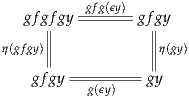
Thus, canceling all but the right-hand homotopy, we have g(ϵy) = η(gy) as desired. __
However, it is important that we do not include both τ and υ in the definition of ishae(f) (whence the name “half adjoint equivalence”). If we did, then after canceling contractible types we would still have one remaining datum — unless we added another higher coherence condition. In general, we expect to get a well-behaved type if we cut off after an odd number of coherences.
Of course, it is obvious that ishae(f) →qinv(f): simply forget the coherence datum. The other direction is a version of a standard argument from homotopy theory and category theory.
Proof. Suppose that (g, η, ϵ) is a quasi-inverse for f. We have to provide a quadruple (g′, η′, ϵ′, τ) witnessing that f is a half adjoint equivalence. To define g′ and η′, we can just make the obvious choice by setting g′:≡ g and η′:≡ η. However, in the definition of ϵ′ we need start worrying about the construction of τ, so we cannot just follow our nose and take ϵ′ to be ϵ. Instead, we take
 |
Now we need to find
 |
Note first that by Corollary 2.4.4, we have η(g(f(a))) = g .
Therefore, we can apply Lemma 2.4.3 to compute
.
Therefore, we can apply Lemma 2.4.3 to compute
f ▪ϵ(f(a)) ▪ϵ(f(a)) | = f ▪ϵ(f(a)) ▪ϵ(f(a)) | ||
= ϵ(f(g(f(a)))) ▪f |
Combining this with Lemma 4.2.2 (or symmetrizing the proof), we also have qinv(f) →ishae′(f).
It remains to show that ishae(f) is a mere proposition. For this, we will need to know that the fibers of an equivalence are contractible.
In homotopy theory, this is what would be called the homotopy fiber of f. The path lemmas in §2.5 yield the following characterization of paths in fibers:
Theorem 4.2.6. If f : A → B is a half adjoint equivalence, then for any y : B the fiber fibf(y) is contractible.
Proof. Let (g, η, ϵ, τ) : ishae(f), and fix y : B. As our center of contraction for
fibf(y) we choose (gy, ϵy). Now take any (x, p) : fibf(y); we want to construct
a path from (gy, ϵy) to (x, p). By Lemma 4.2.5, it suffices to give a path
γ : gy = x such that f ▪p = ϵy. We put γ :≡ g(p)-1 ▪ηx. Then we
have
▪p = ϵy. We put γ :≡ g(p)-1 ▪ηx. Then we
have
| f(γ) ▪p | = fg(p)-1 ▪f(ηx) ▪p | ||
| = fg(p)-1 ▪ϵ(fx) ▪p | |||
| = ϵy |
We now define the types which encapsulate contractible pairs of data. The following types put together the quasi-inverse g with one of the homotopies.
Definition 4.2.7. Given a function f : A → B, we define the types
| linv(f) | :≡ ∑ g:B→A (g∘f ~idA) | ||
| rinv(f) | :≡ ∑ g:B→A (f ∘g ~idB) |
Lemma 4.2.8. If f : A → B has a quasi-inverse, then so do
| (f ∘–) | : (C → A) → (C → B) | ||
| (– ∘f) | : (B → C) → (A → C). |
Proof. If g is a quasi-inverse of f, then (g ∘ –) and (– ∘ g) are quasi-inverses of (f ∘ –) and (– ∘f) respectively. __
Proof. By function extensionality, we have
But this is the fiber of (– ∘ f) over idA, and so by Lemma 4.2.8 and Theorems 4.2.3 and 4.2.6, it is contractible. Similarly, rinv(f) is equivalent to the fiber of (f ∘ –) over idB and hence contractible. __
Next we define the types which put together the other homotopy with the additional coherence datum.
Definition 4.2.10. For f : A → B, a left inverse (g, η) : linv(f), and a right inverse (g, ϵ) : rinv(f), we denote
| lcohf(g, η) | :≡ ∑ (ϵ:f∘g~idB) ∏ (y:B) g(ϵy) = η(gy), | ||
| rcohf(g, ϵ) | :≡ ∑ (η:g∘f~idA) ∏ (x:A) f(ηx) = ϵ(fx). |
Lemma 4.2.11. For any f, g, ϵ, η, we have
| lcohf(g, η) | ≃ ∏ y:B (fgy, η(gy)) =fibg(gy) (y, reflgy), | ||
| rcohf(g, ϵ) | ≃ ∏ x:A (gfx, ϵ(fx)) =fibf(fx) (x, reflfx). |
Proof. Using Lemma 4.2.5. __
Lemma 4.2.12. If f is a half adjoint equivalence, then for any (g, ϵ) : rinv(f), the type rcohf(g, ϵ) is contractible.
Proof. By Lemma 4.2.11 and the fact that dependent function types preserve contractible spaces, it suffices to show that for each x : A, the type (gfx, ϵ(fx)) =fibf(fx) (x, reflfx) is contractible. But by Theorem 4.2.6, fibf(fx) is contractible, and any path space of a contractible space is itself contractible. __
Proof. By Exercise 3.5 it suffices to assume f to be a half adjoint equivalence and show that ishae(f) is contractible. Now by associativity of Σ (Exercise 2.10), the type ishae(f) is equivalent to
But by Lemmas 4.2.9 and 4.2.12 and the fact that Σ preserves contractibility, the latter type is also contractible. __
Thus, we have shown that ishae(f) has all three desiderata for the type isequiv(f). In the next two sections we consider a couple of other possibilities.
Using the language introduced in §4.2, we can restate the definition proposed in §2.4 as follows.
Definition 4.3.1. We say f : A → B is bi-invertible if it has both a left inverse and a right inverse:
In §2.4 we proved that qinv(f) →biinv(f) and biinv(f) →qinv(f). What remains is the following.
Proof. We may suppose f to be bi-invertible and show that biinv(f) is contractible. But since biinv(f) →qinv(f), by Lemma 4.2.9 in this case both linv(f) and rinv(f) are contractible, and the product of contractible types is contractible. __
Note that this also fits the proposal made at the beginning of §4.2: we combine g and η into a contractible type and add an additional datum which combines with ϵ into a contractible type. The difference is that instead of adding a higher datum (a 2-dimensional path) to combine with ϵ, we add a lower one (a right inverse that is separate from the left inverse).
Proof. We have biinv(f) → qinv(f) → ishae(f) and ishae(f) → qinv(f) → biinv(f). Since both ishae(f) and biinv(f) are mere propositions, the equivalence follows from Lemma 3.3.3. __
Note that our proofs about ishae(f) and biinv(f) made essential use of the fact that the fibers of an equivalence are contractible. In fact, it turns out that this property is itself a sufficient definition of equivalence.
Definition 4.4.1 (Contractible maps). A map f : A → B is contractible if for all y : B, the fiber fibf(y) is contractible.
Thus, the type isContr(f) is defined to be
| isContr(f) | :≡ ∏ y:B isContr(fibf(y)) | (4.4.2) |
We have already shown in Theorem 4.2.6 that ishae(f) →isContr(f). Conversely:
Proof. Let P : isContr(f). We define an inverse mapping g : B → A by sending each y : B to the center of contraction of the fiber at y:
We can thus define the homotopy ϵ by mapping y to the witness that g(y) indeed belongs to the fiber at y:
It remains to define η and τ. This of course amounts to giving an element of rcohf(g, ϵ). By Lemma 4.2.11, this is the same as giving for each x : A a path from (gfx, ϵ(fx)) to (x, reflfx) in the fiber of f over fx. But this is easy: for any x : A, the type fibf(fx) is contractible by assumption, hence such a path must exist. We can construct it explicitly as

It is also easy to see:
Proof. By Lemma 3.11.4, each type isContr(fibf(y)) is a mere proposition. Thus, by Example 3.6.2, so is (4.4.2). __
Proof. We have already established a logical equivalence isContr(f) ⇔ ishae(f), and both are mere propositions (Lemma 4.4.4 and Theorem 4.2.13). Thus, Lemma 3.3.3 applies. __
Usually, we prove that a function is an equivalence by exhibiting a quasi-inverse, but sometimes this definition is more convenient. For instance, it implies that when proving a function to be an equivalence, we are free to assume that its codomain is inhabited.
Proof. To show f is an equivalence, it suffices to show that fibf(y) is contractible for any y : B. But if e : B →isequiv(f), then given any such y we have e(y) : isequiv(f), so that f is an equivalence and hence fibf(y) is contractible, as desired. __
We have shown that all three definitions of equivalence satisfy the three desirable properties and are pairwise equivalent:

(There are yet more possible definitions of equivalence, but we will stop with these three. See Exercise 3.8 and the exercises in this chapter for some more.) Thus, we may choose any one of them as “the” definition of isequiv(f). For definiteness, we choose to define
This choice is advantageous for formalization, since ishae(f) contains the most directly useful data. On the other hand, for other purposes, biinv(f) is often easier to deal with, since it contains no 2-dimensional paths and its two symmetrical halves can be treated independently. However, for purposes of this book, the specific choice will make little difference.
In the rest of this chapter, we study some other properties and characterizations of equivalences.
When A and B are sets and f : A → B is an equivalence, we also call it as isomorphism or a bijection. (We avoid these words for types that are not sets, since in homotopy theory and higher category theory they often denote a stricter notion of “sameness” than homotopy equivalence.) In set theory, a function is a bijection just when it is both injective and surjective. The same is true in type theory, if we formulate these conditions appropriately. For clarity, when dealing with types that are not sets, we will speak of embeddings instead of injections.
In other words, f is surjective if every fiber of f is merely inhabited, or equivalently if for all b : B there merely exists an a : A such that f(a) = b. In traditional logical notation, f is surjective if ∀(b : B).∃(a : A).(f(a) = b). This must be distinguished from the stronger assertion that ∏(b:B) ∑(a:A) (f(a) = b); if this holds we say that f is a split surjection.
If A and B are sets, then by Lemma 3.3.3, f is an embedding just when
 | (4.6.2) |
In this case we say that f is injective, or an injection. We avoid these word for types that are not sets, because they might be interpreted as (4.6.2), which is an ill-behaved notion for non-sets. It is also true that any function between sets is surjective if and only if it is an epimorphism in a suitable sense, but this also fails for more general types, and surjectivity is generally the more important notion.
Theorem 4.6.3. A function f : A → B is an equivalence if and only if it is both surjective and an embedding.
Proof. If f is an equivalence, then each fibf(b) is contractible, hence so is
 , so f is surjective. And we showed in Theorem 2.11.1 that any
equivalence is an embedding.
, so f is surjective. And we showed in Theorem 2.11.1 that any
equivalence is an embedding.
Conversely, suppose f is a surjective embedding. Let b : B; we show
that ∑(x:A) (f(x) = b) is contractible. Since f is surjective, there merely
exists an a : A such that f(a) = b. Thus, the fiber of f over b is inhabited;
it remains to show it is a mere proposition. For this, suppose given
x, y : A with p : f(x) = b and q : f(y) = b. Then since apf is an
equivalence, there exists r : x = y with apf(r) = p▪q-1. However, using
the characterization of paths in Σ-types, the latter equality rearranges to
r* = q. Thus, together with r it exhibits (x, p) = (y, q) in the fiber of
f over b. __
= q. Thus, together with r it exhibits (x, p) = (y, q) in the fiber of
f over b. __
Proof. Being a surjection and an embedding are both mere propositions; now apply Lemma 3.3.3. __
Of course, this cannot be used as a definition of “equivalence”, since the definition of embeddings refers to equivalences. However, this characterization can still be useful; see §8.8. We will generalize it in Chapter 7.
We have already seen in Lemma 2.4.12 that equivalences are closed under composition. Furthermore, we have:
Theorem 4.7.1 (The 2-out-of-3 property). Suppose f : A → B and g : B → C. If any two of f, g, and g∘f are equivalences, so is the third.
Proof. If g∘f and g are equivalences, then (g∘f)-1 ∘g is a quasi-inverse to f. On the one hand, we have (g∘f)-1 ∘g∘f ~id A, while on the other we have
| f ∘ (g∘f)-1 ∘g | ~ g-1 ∘g∘f ∘ (g∘f)-1 ∘g | ||
| ~ g-1 ∘g | |||
| ~idB. |
This is a standard closure condition on equivalences from homotopy theory. Also well-known is that they are closed under retracts, in the following sense.
Definition 4.7.2. A function g : A → B is said to be a retract of a function f : X → Y if there is a diagram
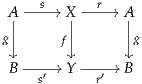 |
for which there are
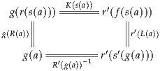 |
Recall that in §3.11 we defined what it means for a type to be a retract of another. This is a special case of the above definition where B and Y are 1. Conversely, just as with contractibility, retractions of maps induce retractions of their fibers.
Lemma 4.7.3. If a function g : A → B is a retract of a function f : X → Y, then fibg(b) is a retract of fibf(s′(b)) for every b : B, where s′ : B → Y is as in Definition 4.7.2.
Proof. Suppose that g : A → B is a retract of f : X → Y. Then for any b : B we have the functions
| φb | : fibg(b) →fibf(s′(b)), | φb(a, p) | :≡ (s(a), L(a) ▪s′(p)), | ||||
| ψb | : fibf(s′(b)) →fibg(b), | ψb(x, q) | :≡ (r(x), K(x) ▪r′(q) ▪R′(b)). |
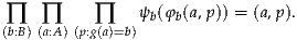 |
By reordering the first two Πs and applying a version of Lemma 3.11.9, this is equivalent to
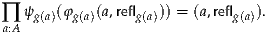 |
For any a, by Theorem 2.7.2, this equality of pairs is equivalent to a pair of equalities. The first components are equal by R(a) : r(s(a)) = a, so we need only show
 |
But this transportation computes as g(R(a))-1 ▪K(s(a)) ▪r′(L(a)) ▪R′(g(a)), so the required path is given by H(a). __
Proof. By Lemma 4.7.3, every fiber of g is a retract of a fiber of f. Thus, by Lemma 3.11.7, if the latter are all contractible, so are the former. __
Finally, we show that fiberwise equivalences can be characterized in terms
of equivalences of total spaces. To explain the terminology, recall from §2.3
that a type family P : A → can be viewed as a fibration over A with total
space ∑(x:A) P(x), the fibration being is the projection pr1 : ∑(x:A) P(x) → A.
From this point of view, given two type families P, Q : A →, we may
refer to a function f : ∏(x:A) (P(x) → Q(x)) as a fiberwise map or a
fiberwise transformation. Such a map induces a function on total
spaces:
Theorem 4.7.6. Suppose that f is a fiberwise transformation between families P and Qover a type Aand let x : Aand v : Q(x). Then we have an equivalence
 |
Proof. We calculate:
| fibtotal(f)((x, v)) | ≡ ∑ w:∑(x:A) P(x) (pr1w, f(pr1w, pr2w)) = (x, v) | ||
| ≃ ∑ (a:A) ∑ (u:P(a)) (a, f(a, u)) = (x, v) | (by Exercise 2.10) | ||
≃ ∑
(a:A) ∑
(u:P(a)) ∑
(p:a=x) p* = v = v | (by Theorem 2.7.2) | ||
≃ ∑
(a:A) ∑
(p:a=x) ∑
(u:P(a)) p* = v = v | |||
| ≃ ∑ u:P(x) f(x, u) = v | (*) | ||
| ≡fibf(x)(v). |
We say that a fiberwise transformation f : ∏(x:A) P(x) → Q(x) is a fiberwise equivalence if each f(x) : P(x) → Q(x) is an equivalence.
Theorem 4.7.7. Suppose that f is a fiberwise transformation between families P and Qover a type A. Then f is a fiberwise equivalence if and only if total(f) is an equivalence.
Proof. Let f, P, Q and A be as in the statement of the theorem. By Theorem 4.7.6 it follows for all x : A and v : Q(x) that fibtotal(f)((x, v)) is contractible if and only if fibf(x)(v) is contractible. Thus, fibtotal(f)(w) is contractible for all w : ∑(x:A) Q(x) if and only if fibf(x)(v) is contractible for all x : A and v : Q(x). __
In type theory we have a basic notion of family of types, namely a function
B : A →. We have seen that such families behave somewhat like
fibrations in homotopy theory, with the fibration being the projection
pr1 : ∑(a:A) B(a) → A. A basic fact in homotopy theory is that every map is
equivalent to a fibration. With univalence at our disposal, we can prove the
same thing in type theory.
Lemma 4.8.1. For any type family B : A → , the fiber of pr1 :
∑
(x:A) B(x) → Aover a : Ais equivalent to B(a):
Proof. We have
| fibpr1 (a) | :≡ ∑ u:∑(x:A) B(x) pr1(u) = a | ||
| ≃ ∑ (x:A) ∑ (b:B(x)) (x = a) | |||
| ≃ ∑ (x:A) ∑ (p:x=a) B(x) | |||
| ≃ B(a) |
Proof. We have
| ∑ b:B fibf(b) | :≡ ∑ (b:B) ∑ (a:A) (f(a) = b) | ||
| ≃ ∑ (a:A) ∑ (b:B) (f(a) = b) | |||
| ≃ A |
Proof. We have to construct quasi-inverses
| χ | :  ∑
A: (A → B) ∑
A: (A → B) → B → → B → | ||
| ψ | : (B →) → ∑
A: (A → B) ∑
A: (A → B) . . |
 .
Now we have to verify that χ∘ψ ~id and that ψ∘χ ~id.
. By Lemma 4.8.1, fibpr1 (b) ≃ P(b) for any b : B, so it
follows immediately that P ~ χ(ψ(P)).
.
Now we have to verify that χ∘ψ ~id and that ψ∘χ ~id.
. By Lemma 4.8.1, fibpr1 (b) ≃ P(b) for any b : B, so it
follows immediately that P ~ χ(ψ(P)).
 |
First note that by Lemma 4.8.2, we have e : ∑(b:B) fibf(b) ≃ A with
e(b, a, p) :≡ a and e-1(a) :≡ (f(a), a, reflf(a)). By Theorem 2.7.2, it
remains to show (ua(e))* = f. But by the computation rule for
univalence and (2.9.4), we have (ua(e))*
= f. But by the computation rule for
univalence and (2.9.4), we have (ua(e))* = pr1 ∘e-1, and the
definition of e-1 immediately yields pr1 ∘e-1 ≡ f. __
= pr1 ∘e-1, and the
definition of e-1 immediately yields pr1 ∘e-1 ≡ f. __
In particular, this implies that we have an object classifier in the sense of higher
topos theory. Recall from Definition 2.1.7 that ∙ denotes the type ∑(A:) A of
pointed types.
Theorem 4.8.4. Let f : A → B be a function. Then the diagram
 |
is a pullback square (see Exercise 2.11). Here the function ϑf is defined by
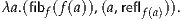 |
Proof. Note that we have the equivalences
| A | ≃ ∑ b:B fibf(b) | ||
| ≃ ∑
(b:B) ∑
(X:) ∑
(p:fibf(b)=X) X | |||
| ≃ ∑
(b:B) ∑
(X:) ∑
(x:X) fibf(b) = X | |||
| ≃ ∑
(b:B) ∑
(Y:∙) fibf(b) = pr1Y | |||
| ≡ B×∙. |
∙. We may display the
action of this composite equivalence step by step by
| a |  (f(a), (a, reflf(a))) (f(a), (a, reflf(a))) | ||
 (f(a), fibf(f(a)), reflfibf(f(a)), (a, reflf(a))) (f(a), fibf(f(a)), reflfibf(f(a)), (a, reflf(a))) | |||
 (f(a), fibf(f(a)), (a, reflf(a)), reflfibf(f(a))). (f(a), fibf(f(a)), (a, reflf(a)), reflfibf(f(a))). |
In the last section of this chapter we include a proof that the univalence axiom implies function extensionality. Thus, in this section we work without the function extensionality axiom. The proof consists of two steps. First we show in Theorem 4.9.4 that the univalence axiom implies a weak form of function extensionality, defined in Definition 4.9.1 below. The principle of weak function extensionality in turn implies the usual function extensionality, and it does so without the univalence axiom (Theorem 4.9.5).
Let be a universe; we will explicitly indicate where we assume that it is
univalent.
Definition 4.9.1. The weak function extensionality principle asserts that there is a function
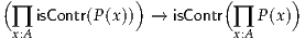 |
for any family P : A → of types over any type A.
The following lemma is easy to prove using function extensionality; the point here is that it also follows from univalence without assuming function extensionality separately.
Lemma 4.9.2. Assuming is univalent, for any A, B, X : and any e : A ≃ B,
there is an equivalence
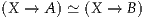 |
of which the underlying map is given by post-composition with the underlying function of e.
Proof. As in the proof of Lemma 4.1.1, we may assume that e = idtoeqv(p) for some p : A = B. Then by path induction, we may assume p is reflA, so that e = idA. But in this case, post-composition with e is the identity, hence an equivalence. __
Corollary 4.9.3. Let P : A →be a family of contractible types, i.e.
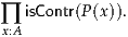 |
Then the projection pr1 : ( ∑(x:A) P(x)) → Ais an equivalence. Assuming is
univalent, it follows immediately that post-composition with pr1 gives an
equivalence
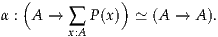 |
Proof. By Lemma 4.8.1, for pr1 : ∑(x:A) P(X) → A and x : A we have an equivalence
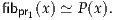 |
Therefore pr1 is an equivalence whenever each P(x) is contractible. The assertion is now a consequence of Lemma 4.9.2. __
In particular, the homotopy fiber of the above equivalence at idA is contractible. Therefore, we can show that univalence implies weak function extensionality by showing that the dependent function type ∏(x:A) P(x) is a retract of fibα(idA).
Theorem 4.9.4. In a univalent universe , suppose that P : A → is
a family of contractible types and let α be the function of Corollary 4.9.3.
Then ∏(x:A) P(x) is a retract of fibα(idA). As a consequence, ∏(x:A) P(x) is
contractible. In other words, the univalence axiom implies the weak function
extensionality principle.
Proof. Define the functions
| φ | : ∏(x:A)P(x) →fibα(idA), | ||
| φ(f) | :≡ (λx.(x, f(x)), reflidA), | ||
| and | |||
| ψ | : fibα(idA) →∏(x:A)P(x), | ||
| ψ(g, p) | :≡ λx.p* . . | ||
We now show that weak function extensionality implies the usual function extensionality. Recall from (2.9.2) the function happly(f, g) : (f = g) → (f ~ g) which converts equality of functions to homotopy. In the proof that follows, the univalence axiom is not used.
Theorem 4.9.5. Weak function extensionality implies the function extensionality Axiom 2.9.3.
Proof. We want to show that
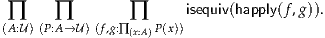 |
Since a fiberwise map induces an equivalence on total spaces if and only if it is fiberwise an equivalence by Theorem 4.7.7, it suffices to show that the function of type
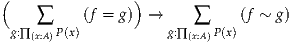 |
induced by λ(g: ∏(x:A) P(x)).happly(f, g) is an equivalence. Since the type on the left is contractible by Lemma 3.11.8, it suffices to show that the type on the right:
 | (4.9.6) |
is contractible. Now Theorem 2.15.7 says that this is equivalent to
 | (4.9.7) |
The proof of Theorem 2.15.7 uses function extensionality, but only for one of the composites. Thus, without assuming function extensionality, we can conclude that (4.9.6) is a retract of (4.9.7). And (4.9.7) is a product of contractible types, which is contractible by the weak function extensionality principle; hence (4.9.6) is also contractible. __
The fact that the space of continuous maps equipped with quasi-inverses has
the wrong homotopy type to be the “space of homotopy equivalences” is
well-known in algebraic topology. In that context, the “space of homotopy
equivalences” (A ≃ B) is usually defined simply as the subspace of the
function space (A → B) consisting of the functions that are homotopy
equivalences. In type theory, this would correspond most closely to
∑
(f:A→B)  ; see Exercise 3.8.
The first definition of equivalence given in homotopy type theory was the one that we have called isContr(f), which was due to Voevodsky. The possibility of the other definitions was subsequently observed by various people. The basic theorems about adjoint equivalences such as Lemma 4.2.2 and Theorem 4.2.3 are adaptations of standard facts in higher category theory and homotopy theory. Using bi-invertibility as a definition of equivalences was suggested by André Joyal.
The properties of equivalences discussed in §§4.6 and 4.7 are well-known in homotopy theory. Most of them were first proven in type theory by Voevodsky.
The fact that every function is equivalent to a fibration is a standard fact in homotopy theory. The notion of object classifier in (∞, 1)-category theory (the categorical analogue of Theorem 4.8.3) is due to Rezk (see [Rez05, Lur09]).
Finally, the fact that univalence implies function extensionality (§4.9) is due to Voevodsky. Our proof is a simplification of his.
Exercise 4.1. Consider the type of “two-sided adjoint equivalence data” for f : A → B,
Can you give an example showing that this type is not generally a mere proposition? (This will be easier after Chapter 6.)
Exercise 4.2. Show that for any A, B : , the following type is equivalent to
A ≃ B.
 |
Can you extract from this a definition of a type satisfying the three desiderata of isequiv(f)?
Exercise 4.3. Reformulate the proof of Lemma 4.1.1 without using univalence.
Exercise 4.4 (The unstable octahedral axiom). Suppose f : A → B and g : B → C and b : B.
Exercise 4.5. Prove that equivalences satisfy the 2-out-of-6 property: given f : A → B and g : B → C and h : C → D, if g ∘f and h∘g are equivalences, so are f, g, h, and h∘g∘f. Use this to give a higher-level proof of Theorem 2.11.1.
Exercise 4.6. For A, B : , define
by path induction in the obvious way. Let qinv-univalence denote the
modified form of the univalence axiom which asserts that for all A, B : the
function idtoqinvA,B has a quasi-inverse.
In Chapter 1, we introduced many ways to form new types from old ones. Except for (dependent) function types and universes, all these rules are special cases of the general notion of inductive definition. In this chapter we study inductive definitions more generally.
An inductive type X can be intuitively understood as a type “freely generated” by a certain finite collection of constructors, each of which is a function (of some number of arguments) with codomain X. This includes functions of zero arguments, which are simply elements of X.
When describing a particular inductive type, we list the constructors with bullets. For instance, the type 2 from §1.8 is inductively generated by the following constructors:
Similarly, 1 is inductively generated by the constructor:
while 0 is inductively generated by no constructors at all. An example where the constructor functions take arguments is the coproduct A + B, which is generated by the two constructors
And an example with a constructor taking multiple arguments is the cartesian product A×B, which is generated by one constructor
Crucially, we also allow constructors of inductive types that take arguments from the inductive type being defined. For instance, the type N of natural numbers has constructors
Another useful example is the type List(A) of finite lists of elements of some type A, which has constructors
Intuitively, we should understand an inductive type as being freely generated by its constructors. That is, the elements of an inductive type are exactly what can be obtained by starting from nothing and applying the constructors repeatedly. (We will see in §5.8 and Chapter 6 that this conception has to be modified slightly for more general kinds of inductive definitions, but for now it is sufficient.) For instance, in the case of 2, we should expect that the only elements are 02 and 12. Similarly, in the case of N, we should expect that every element is either 0 or obtained by applying succ to some “previously constructed” natural number.
Rather than assert properties such as this directly, however, we express them by means of an induction principle, also called a (dependent) elimination rule. We have seen these principles already in Chapter 1. For instance, the induction principle for 2 is:
about all inhabitants of 2, it
suffices to prove it for 02 and 12, i.e., to give proofs e0 : E(02) and
e1 : E(12).Furthermore, the resulting proof ind2(E, e0, e1) : ∏(b:2) E(b) behaves as expected when applied to the constructors 02 and 12; this principle is expressed by the computation rules:
Thus, the induction principle for the type 2 of booleans allow us to reason by case analysis. Since neither of the two constructors takes any arguments, this is all we need for booleans.
For natural numbers, however, case analysis is generally not sufficient: in the case corresponding to the inductive step succ(n), we also want to presume that the statement being proven has already been shown for n. This gives us the following induction principle:
about all natural numbers,
it suffices to prove it for 0 and for succ(n), assuming it holds for n,
i.e., we construct ez : E(0) and es : ∏(n:N) E(n) → E(succ(n)).The variable y represents our inductive hypothesis. As in the case of booleans, we also have the associated computation rules for the function indN(E, ez, es) : ∏(x:N) E(x):
The dependent function indN(E, ez, es) can thus be understood as being defined recursively on the argument x : N, via the functions ez and es which we call the recurrences. When x is zero, the function simply returns ez. When x is the successor of another natural number n, the result is obtained by taking the recurrence es and substituting the specific predecessor n and the recursive call value indN(E, ez, es, n).
The induction principles for all the examples mentioned above share this family resemblance. In §5.6 we will discuss a general notion of “inductive definition” and how to derive an appropriate induction principle for it, but first we investigate various commonalities between inductive definitions.
For instance, we have remarked in every case in Chapter 1 that from the induction principle we can derive a recursion principle in which the codomain is a simple type (rather than a family). Both induction and recursion principles may seem odd, since they yield only the existence of a function without seeming to characterize it uniquely. However, in fact the induction principle is strong enough also to prove its own uniqueness principle, as in the following theorem.
Theorem 5.1.1. Let f, g : ∏(x:N) E(x) be two functions which satisfy the recurrences
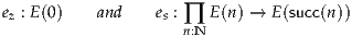 |
up to propositional equality, i.e., such that
 |
as well as
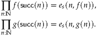
Proof. We use induction on the type family D(x) :≡ f(x) = g(x). For the base case, we have
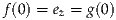
For the inductive case, assume n : N such that f(n) = g(n). Then

The first and last equality follow from the assumptions on f and g. The middle equality follows from the inductive hypothesis and the fact that application preserves equality. This gives us pointwise equality between f and g; invoking function extensionality finishes the proof. __
Note that the uniqueness principle applies even to functions that only satisfy the recurrences up to propositional equality, i.e. a path. Of course, the particular function obtained from the induction principle satisfies these recurrences judgmentally; we will return to this point in §5.5. On the other hand, the theorem itself only asserts a propositional equality between functions (see also Exercise 5.2). From a homotopical viewpoint it is natural to ask whether this path is coherent, i.e. whether the equality f = g is unique up to higher paths; in §5.4 we will see that this is in fact the case.
Of course, similar uniqueness theorems for functions can generally be formulated and shown for other inductive types as well. In the next section, we show how this uniqueness property, together with univalence, implies that an inductive type such as the natural numbers is completely characterized by its introduction, elimination, and computation rules.
We have defined “the” natural numbers to be a particular type N with particular inductive generators 0 and succ. However, by the general principle of inductive definitions in type theory described in the previous section, there is nothing preventing us from defining another type in an identical way. That is, suppose we let N′ be the inductive type generated by the constructors
Then N′ will have identical-looking induction and recursion principles to N.
When proving a statement E : N′→ for all of these “new” natural
numbers, it suffices to give the proofs ez : E(0′) and
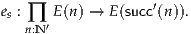 |
And the function recN′(E, ez, es) : ∏(n:N′) E(n) has the following computation rules:
But what is the relation between N and N′?
This is not just an academic question, since structures that “look like” the natural numbers can be found in many other places. For instance, we may identify natural numbers with lists over the type with one element (this is arguably the oldest appearance, found on walls of caves), with the non-negative integers, with subsets of the rationals and the reals, and so on. And from a programming point of view, the “unary” representation of our natural numbers is very inefficient, so we might prefer sometimes to use a binary one instead. We would like to be able to identify all of these versions of “the natural numbers” with each other, in order to transfer constructions and results from one to another.
Of course, if two versions of the natural numbers satisfy identical induction principles, then they have identical induced structure. For instance, recall the example of the function double defined in §1.9. A similar function for our new natural numbers is readily defined by duplication and adding primes:

Simple as this may seem, it has the obvious drawback of leading to a proliferation of duplicates. Not only functions have to be duplicated, but also all lemmas and their proofs. For example, an easy result such as ∏ (n:N) double(succ(n)) = succ(succ(double(n))), as well as its proof by induction, also has to be “primed”.
In traditional mathematics, one just proclaims that N and N′ are obviously “the same”, and can be substituted for each other whenever the need arises. This is usually unproblematic, but it sweeps a fair amount under the rug, widening the gap between informal mathematics and its precise description. In homotopy type theory, we can do better.
First observe that we have the following definable maps:
Since the composition of g and f satisfies the same recurrences as the identity function on N, Theorem 5.1.1 gives that ∏(n:N) g(f(n)) = n, and the “primed” version of the same theorem gives ∏(n:N′) f(g(n)) = n. Thus, f and g are quasi-inverses, so that N ≃N′. We can now transfer functions on N directly to functions on N′ (and vice versa) along this equivalence, e.g.

It is an easy exercise to show that this version of double′ is equal to the earlier one.
Of course, there is nothing surprising about this; such an isomorphism is exactly how a mathematician will envision “identifying” N with N′. However, the mechanism of “transfer” across an isomorphism depends on the thing being transferred; it is not always as simple as pre- and post-composing a single function with f and g. Consider, for instance, a simple lemma such as
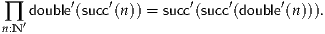
Inserting the correct fs and gs is only a little easier than re-proving it by induction on n : N′ directly.
Here is where the univalence axiom steps in: since N ≃N′, we also have
N = N′, i.e. N and N′ are equal as types. Now the induction principle
for identity guarantees that any construction or proof relating to N
can automatically be transferred to N′ in the same way. We simply
consider the type of the function or theorem as a type-indexed family of
types P : →, with the given object being an element of P(N), and
transport along the path N = N′. This involves considerably less
overhead.
For simplicity, we have described this method in the case of two types N and N′ with identical-looking definitions. However, a more common situation in practice is when the definitions are not literally identical, but nevertheless one induction principle implies the other. Consider, for instance, the type of lists from a one-element type, List(1), which is generated by
This is not identical to the definition of N, and it does not give rise to an identical
induction principle. The induction principle of List(1) says that for
any E : List(1) → together with recurrence data enil : E(nil) and
econs : ∏(u:1) ∏(ℓ:List(1)) E(ℓ) → E(cons(u, ℓ)), there exists f : ∏(ℓ:List(1)) E(ℓ)
such that f(nil) ≡ enil and f(cons(u, ℓ)) ≡ econs(u, ℓ, f(ℓ)). (We will see
how to derive the induction principle of an inductive definition in
§5.6.)
Now suppose we define 0′′:≡nil : List(1), and succ′′ : List(1) →List(1) by
succ′′(ℓ) :≡cons(⋆, ℓ). Then for any E : List(1) → together with e0 : E(0′′)
and es : ∏(ℓ:List(1)) E(ℓ) → E(succ′′(ℓ)), we can define
| enil | :≡ e0 | ||
| econs(⋆, ℓ, x) | :≡ es(ℓ, x). |
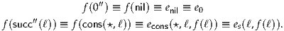
Finally, these conclusions are not confined to the natural numbers: they
apply to any inductive type. If we have an inductively defined type W, say,
and some other type W′ which satisfies the same induction principle as W,
then it follows that W ≃ W′, and hence W = W′. We use the derived recursion
principles for W and W′ to construct maps W → W′ and W′→ W,
respectively, and then the induction principles for each to prove that both
composites are equal to identities. For instance, in Chapter 1 we saw that the
coproduct A + B could also have been defined as ∑(x:2) rec2(, A, B, x). The
latter type satisfies the same induction principle as the former; hence they are
canonically equivalent.
This is, of course, very similar to the familiar fact in category theory that if two objects have the same universal property, then they are equivalent. In §5.4 we will see that inductive types actually do have a universal property, so that this is a manifestation of that general principle.
Inductive types are very general, which is excellent for their usefulness and applicability, but makes them difficult to study as a whole. Fortunately, they can all be formally reduced to a few special cases. It is beyond the scope of this book to discuss this reduction — which is anyway irrelevant to the mathematician using type theory in practice — but we will take a little time to discuss the one of the basic special cases that we have not yet met. These are Martin-Löf’s W-types, also known as the types of well-founded trees. W-types are a generalization of such types as natural numbers, lists, and binary trees, which are sufficiently general to encapsulate the “recursion” aspect of any inductive type.
A particular W-type is specified by giving two parameters A : and
B : A →, in which case the resulting W-type is written W(a:A)B(a). The
type A represents the type of labels for W(a:A)B(a), which function as
constructors (however, we reserve that word for the actual functions which
arise in inductive definitions). For instance, when defining natural
numbers as a W-type, the type A would be the type 2 inhabited by the
two elements 02 and 12, since there are precisely two ways to obtain a
natural number — either it will be zero or a successor of another natural
number.
The type family B : A → is used to record the arity of labels: a label a : A
will take a family of inductive arguments, indexed over B(a). We can
therefore think of the “B(a)-many” arguments of a. These arguments are
represented by a function f : B(a) →W(a:A)B(a), with the understanding that
for any b : B(a), f(b) is the “b-th” argument to the label a. The W-type
W(a:A)B(a) can thus be thought of as the type of well-founded trees, where
nodes are labeled by elements of A and each node labeled by a : A has
B(a)-many branches.
In the case of natural numbers, the label 02 has arity 0, since it constructs
the constant zero; the label 12 has arity 1, since it constructs the successor of its
argument. We can capture this by using simple elimination on 2 to define a
function rec2(, 0, 1) into a universe of types; this function returns the
empty type 0 for 02 and the unit type 1 for 12. We can thus define
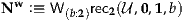
where the superscript w serves to distinguish this version of natural numbers from the previously used one. Similarly, we can define the type of lists over A as a W-type with 1 + A many labels: one nullary label for the empty list, plus one unary label for each a : A, corresponding to appending a to the head of a list:

In general, the W-type W(x:A)B(x) specified by A : and B : A → is the
inductive type generated by the following constructor:
 B(a) →W(x:A)B(x)
 →W(x:A)B(x).
The constructor sup (short for supremum) takes a label a : A and a function f : B(a) →W(x:A)B(x) representing the arguments to a, and constructs a new element of W(x:A)B(x). Using our previous encoding of natural numbers as W-types, we can for instance define
 |
Put differently, we use the label 02 to construct 0w. Then, rec2(, 0, 1, 02)
evaluates to 0, as it should since 02 is a nullary label. Thus, we need to
construct a function f : 0 →Nw, which represents the (zero) arguments
supplied to 02. This is of course trivial, using simple elimination on 0 as
shown. Similarly, we can define 1w and a successor function succw
| 1w | :≡sup(12, λx.0w) | ||
| succw | :≡ λn.sup(12, λx.n). |
We have the following induction principle for W-types:
 W(x:A)B(x)
 → about all elements of
the W-type W(x:A)B(x), it suffices to prove it for sup(a, f), assuming it
holds for all f(b) with b : B(a). In other words, it suffices to give a
proof
→ about all elements of
the W-type W(x:A)B(x), it suffices to prove it for sup(a, f), assuming it
holds for all f(b) with b : B(a). In other words, it suffices to give a
proof
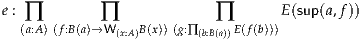 |
The variable g represents our inductive hypothesis, namely that all arguments of a satisfy E. To state this, we quantify over all elements of type B(a), since each b : B(a) corresponds to one argument f(b) of a.
How would we define the function double on natural numbers encoded as a W-type? We would like to use the recursion principle of Nw with a codomain of Nw itself. We thus need to construct a suitable function
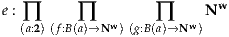
which will represent the recurrence for the double function; for simplicity we
denote the type family rec2(, 0, 1) by B.
Clearly, e will be a function taking a : 2 as its first argument. The next step is to perform case analysis on a and proceed based on whether it is 02 or 12. This suggests the following form
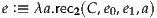
where
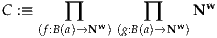
If a is 02, the type B(a) becomes 0. Thus, given f : 0 →Nw and g : 0 →Nw, we want to construct an element of Nw. Since the label 02 represents 0, it needs zero inductive arguments and the variables f and g are irrelevant. We return 0w as a result:
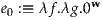
Analogously, if a is 12, the type B(a) becomes 1. Since the label 12 represents the successor operator, it needs one inductive argument — the predecessor — which is represented by the variable f : 1 →Nw. The value of the recursive call on the predecessor is represented by the variable g : 1 →Nw. Thus, taking this value (namely g(⋆)) and applying the successor function twice thus yields the desired result:
 |
Putting this together, we thus have
The associated computation rule for the function rec W(x:A)B(x)(E, e) : ∏(w:W(x:A)B(x)) E(w) is as follows.
 |
In other words, the function recW(x:A)B(x)(E, e) satisfies the recurrence e.
By the above computation rule, the function double behaves as expected:
| double(0w) | ≡recNw(Nw, e, sup(02, λx.rec0(Nw, x))) | ||
≡ e(02,  λx.rec0(Nw, x) λx.rec0(Nw, x) , ,  λx.double(rec0(Nw, x)) λx.double(rec0(Nw, x)) ) ) | |||
≡ e0( λx.rec0(Nw, x) λx.rec0(Nw, x) , ,  λx.double(rec0(Nw, x)) λx.double(rec0(Nw, x)) ) ) | |||
| ≡ 0w | |||
| and | |||
| double(1w) | ≡recNw(Nw, e, sup(12, λx.0w)) | ||
≡ e(12,  λx.0w λx.0w , ,  λx.double(0w) λx.double(0w) ) ) | |||
≡ e1( λx.0w λx.0w , ,  λx.double(0w) λx.double(0w) ) ) | |||
≡succw(succw (λx.double(0w))(⋆) (λx.double(0w))(⋆) ) ) | |||
| ≡succw(succw(0w)) | |||
Just as for natural numbers, we can prove a uniqueness theorem for W-types:
Theorem 5.3.1. Let g, h : ∏(w:W(x:A)B(x)) E(w) be two functions which satisfy the recurrence
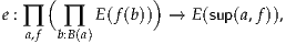 |
propositionally, i.e., such that
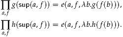
As suggested earlier, inductive types also have a category-theoretic universal property. They are homotopy-initial algebras: initial objects (up to coherent homotopy) in a category of “algebras” determined by the specified constructors. As a simple example, consider the natural numbers. The appropriate sort of “algebra” here is a type equipped with the same structure that the constructors of N give to it.
Definition 5.4.1. A N-algebra is a type C with two elements c0 : C, cs : C → C. The type of such algebras is
 |
Definition 5.4.2. A N-homomorphism between N-algebras (C, c0, cs) and (D, d0, ds) is a function h : C → D such that h(c0) = d0 and h(cs(c)) = ds(h(c)) for all c : C. The type of such homomorphisms is
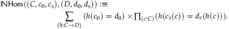
We thus have a category of N-algebras and N-homomorphisms, and the claim is that N is the initial object of this category. A category theorist will immediately recognize this as the definition of a natural numbers object in a category.
Of course, since our types behave like ∞-groupoids, we actually have an (∞, 1)-category of N-algebras, and we should ask N to be initial in the appropriate (∞, 1)-categorical sense. Fortunately, we can formulate this without needing to define (∞, 1)-categories.
Definition 5.4.3. A N-algebra I is called homotopy-initial, or h-initial for short, if for any other N-algebra C, the type of N-homomorphisms from I to C is contractible. Thus,
 |
When they exist, h-initial algebras are unique — not just up to isomorphism, as usual in category theory, but up to equality, by the univalence axiom.
Theorem 5.4.4. Any two h-initial N-algebras are equal. Thus, the type of h-initial N-algebras is a mere proposition.
Proof. Suppose I and J are h-initial N-algebras. Then NHom(I, J) is contractible, hence inhabited by some N-homomorphism f : I → J, and likewise we have an N-homomorphism g : J → I. Now the composite g ∘f is a N-homomorphism from I to I, as is idI; but NHom(I, I) is contractible, so g ∘f = idI. Similarly, f ∘g = idJ. Hence I ≃ J, and so I = J. Since being contractible is a mere proposition and dependent products preserve mere propositions, it follows that being h-initial is itself a mere proposition. Thus any two proofs that I (or J) is h-initial are necessarily equal, which finishes the proof. __
We now have the following theorem.
Sketch of proof. Fix an arbitrary N-algebra (C, c0, cs). The recursion principle of N yields a function f : N → C defined by
| f(0) | :≡ c0 | ||
| f(succ(n)) | :≡ cs(f(n)). |
To place this in a more general context, it is useful to consider the notion of algebra for an endofunctor. Note that to make a type C into a N-algebra is the same as to give a function c : C + 1 → C, and a function f : C → D is a N-homomorphism just when f ∘c ~ d∘ (f + 1). In categorical language, this means the N-algebras are the algebras for the endofunctor F(X) :≡ X + 1 of the category of types.
For a more generic case, consider the W-type associated to A : and
B : A →. In this case we have an associated polynomial functor:
 | (5.4.6) |
Actually, this assignment is functorial only up to homotopy, but this makes no difference in what follows. By definition, a P-algebra is then a type C equipped a function sC : PC → C. By the universal property of Σ-types, this is equivalent to giving a function ∏(a:A) (B(a) → C) → C. We will also call such objects W-algebras for A and B, and we write
 |
Similarly, for P-algebras (C, sC) and (D, sD), a homomorphism between them (f, sf) : (C, sC) → (D, sD) consists of a function f : C → D and a homotopy between maps PC → D
where Pf : PC → PD is the result of the easily-definable action of P on f : C → D. Such an algebra homomorphism can be represented suggestively in the form:
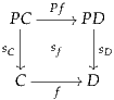 " class="math-display" >
In terms of elements, f is a P-homomorphism (or W-homomorphism) if
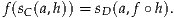
We have the type of W-homomorphisms:
 |
Finally, a P-algebra (C, sC) is said to be homotopy-initial if for every P-algebra (D, sD), the type of all algebra homomorphisms (C, sC) → (D, sD) is contractible. That is,
 |
Now the analogous theorem to Theorem 5.4.5 is:
Theorem 5.4.7. For any type A : and type family B : A → , the
W-algebra (W(x:A)B(x), sup) is h-initial.
Sketch of proof. Suppose we have A : and B : A →, and consider
the associated polynomial functor P(X) :≡ ∑(x:A) (B(x) → X). Let
W :≡W(x:A)B(x). Then using the W-introduction rule from §5.3, we
have a structure map sW :≡sup : PW → W. We want to show that
the algebra (W, sW) is h-initial. So, let us consider another algebra
(C, sC) and show that the type T :≡WHomA,B((W, sW), (C, sC)) of
W-homomorphisms from (W, sW) to (C, sC) is contractible. To do so, observe
that the W-elimination rule and the W-computation rule allow us to
define a W-homomorphism (f, sf) : (W, sW) → (C, sC), thus showing
that T is inhabited. It is furthermore necessary to show that for every
W-homomorphism (g, sg) : (W, sW) → (C, sC), there is an identity
proof
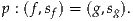 | (5.4.8) |
This uses the fact that, in general, a type of the form (f, sf) = (g, sg) is equivalent to the type of what we call algebra 2-cells, whose canonical elements are pairs of the form (e, se), where e : f = g and se is a higher identity proof between the identity proofs represented by the following pasting diagrams:
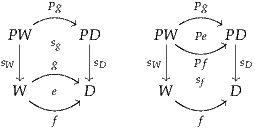
In light of this fact, to prove that there exists an element as in (5.4.8), it is sufficient to show that there is an algebra 2-cell
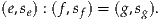
The identity proof e : f = g is now constructed by function extensionality and W-elimination so as to guarantee the existence of the required identity proof se. __
In §5.3 we showed how to encode natural numbers as W-types, with
| Nw | :≡W(b:2)rec2(, 0, 1), | ||
| 0w | :≡sup(02, (λx.rec0(Nw, x))), | ||
| succw | :≡ λn.sup(12, (λx.n)). |
and recurrences
ez : E(0w) and es : ∏(n:Nw) E(n) → E(succw(n)), we can only construct a
dependent function r(E, ez, es) : ∏(n:Nw) E(n) satisfying the given recurrences
propositionally, i.e. up to a path. This means that the computation rules for
natural numbers, which give judgmental equalities, cannot be derived from
the rules for W-types in any obvious way.
This problem goes away if instead of the conventional inductive types we consider homotopy-inductive types, where all computation rules are stated up to a path, i.e. the symbol ≡ is replaced by =. For instance, the computation rule for the homotopy version of W-types Wh becomes:
 |
Homotopy-inductive types have an obvious disadvantage when it comes to computational properties — the behavior of any function constructed using the induction principle can now only be characterized propositionally. But numerous other considerations drive us to consider homotopy-inductive types as well. For instance, while we showed in §5.4 that inductive types are homotopy-initial algebras, not every homotopy-initial algebra is an inductive type (i.e. satisfies the corresponding induction principle) — but every homotopy-initial algebra is a homotopy-inductive type. Similarly, we might want to apply the uniqueness argument from §5.2 when one (or both) of the types involved is only a homotopy-inductive type — for instance, to show that the W-type encoding of N is equivalent to the usual N.
Additionally, the notion of a homotopy-inductive type is now internal to the type theory. For example, this means we can form a type of all natural numbers objects and make assertions about it. In the case of W-types, we can characterize a homotopy W-type W(x:A)B(x) as any type endowed with a supremum function and an induction principle satisfying the appropriate (propositional) computation rule:
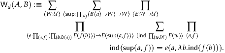 |
In this section, we will state some basic facts about homotopy-inductive types. We omit most of the proofs, which are somewhat technical.
It turns out that there is an equivalent characterization of W-types using a recursion principle, plus certain uniqueness and coherence laws. First we give the recursion principle:
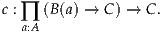 |
The associated computation rule for recWh (x:A)B(x)(C, c) : (W(x:A)B(x)) → C is as follows:
 |
Furthermore, we assert the following uniqueness principle, saying that any two functions defined by the same recurrence are equal:
and c : ∏(a:A) (B(a) → C) → C be given. Let
g, h : (Wh(x:A)B(x)) → C be two functions which satisfy the recurrence c
up to propositional equality, i.e., such that we have
| βg | : ∏ a,f g(sup(a, f)) = c(a, λb.g(f(b))), | ||
| βh | : ∏ a,f h(sup(a, f)) = c(a, λb.h(f(b))). |
Recall that when we have an induction principle rather than only a recursion principle, this propositional uniqueness principle is derivable (Theorem 5.3.1). But with only recursion, the uniqueness principle is no longer derivable — and in fact, the statement is not even true (exercise). Hence, we postulate it as an axiom. We also postulate the following coherence law, which tells us how the proof of uniqueness behaves on canonical elements:
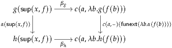
where α abbreviates the path α(C, c, f, g, βg, βh) : g = h.
Putting all of this data together yields another characterization of W(x:A)B(x), as a type with a supremum function, satisfying simple elimination, computation, uniqueness, and coherence rules:
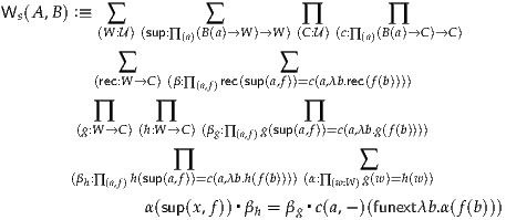 |
Finally, we have a third, very concise characterization of W(x:A)B(x) as an h-initial W-algebra:
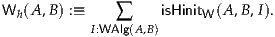 |
It turns out all three characterizations of W-types are in fact equivalent:
Indeed, we have the following theorem, which is an improvement over Theorem 5.4.7:
Theorem 5.5.5. The types satisfying the formation, introduction, elimination, and propositional computation rules for W-types are precisely the homotopy-initial W-algebras.
Sketch of proof. Inspecting the proof of Theorem 5.4.7, we see that
only the propositional computation rule was required to establish the
h-initiality of W(x:A)B(x). For the converse implication, let us assume
that the polynomial functor associated to A : and B : A → , has
an h-initial algebra (W, sW); we show that W satisfies the propositional
rules of W-types. The W-introduction rule is simple; namely, for a : A
and t : B(a) → W, we define sup(a, t) : W to be the result of applying
the structure map sW : PW → W to (a, t) : PW. For the W-elimination
rule, let us assume its premisses and in particular that C′ : W → .
Using the other premisses, one shows that the type C :≡ ∑(w:W) C′(w)
can be equipped with a structure map sC : PC → C. By the h-initiality
of W, we obtain an algebra homomorphism (f, sf) : (W, sW) → (C, sC).
Furthermore, the first projection pr1 : C → W can be equipped with the
structure of a homomorphism, so that we obtain a diagram of the form
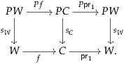
But the identity function 1W : W → W has a canonical structure of an algebra homomorphism and so, by the contractibility of the type of homomorphisms from (W, sW) to itself, there must be an identity proof between the composite of (f, sf) with (pr1, spr1 ) and (1W, s1W). This implies, in particular, that there is an identity proof p : pr1 ∘f = 1W.
Since (pr2 ∘f)w : C((pr1 ∘f)w), we can define

where the transport p* is with respect to the family

The verification of the propositional W-computation rule is a calculation, involving the naturality properties of operations of the form p*. __
Finally, as desired, we can encode homotopy-natural-numbers as homotopy-W-types:
Theorem 5.5.6. The rules for natural numbers with propositional computation rules can be derived from the rules for W-types with propositional computation rules.
So far, we have been discussing only particular inductive types: 0, 1, 2, N, coproducts, products, Σ-types, W-types, etc. However, an important aspect of type theory is the ability to define new inductive types, rather than being restricted only to some particular fixed list of them. In order to be able to do this, however, we need to know what sorts of “inductive definitions” are valid or reasonable.
To see that not everything which “looks like an inductive definition” makes sense, consider the following “constructor” of a type C:
The recursion principle for such a type C ought to say that given a type P, in order to construct a function f : C → P, it suffices to consider the case when the input c : C is of the form g(α) for some α : C →N. Moreover, we would expect to be able to use the “recursive data” of f applied to α in some way. However, it is not at all clear how to “apply f to α”, since both are functions with domain C.
We could write down a “recursion principle” for C by just supposing (unjustifiably) that there is some way to apply f to α and obtain a function P →N. Then the input to the recursion rule would ask for a type P together with a function
 | (5.6.1) |
where the two arguments of h are α and “the result of applying f to α”. However, what would the computation rule for the resulting function f : C → P be? Looking at other computation rules, we would expect something like “f(g(α)) ≡ h(α, f(α))” for α : C →N, but as we have seen, “f(α)” does not make sense. The induction principle of C is even more problematic; it’s not even clear how to write down the hypotheses.
On the other hand, we could write down a different “recursion principle” for C by ignoring the “recursive” presence of C in the domain of α, considering it as merely an indexing type for a family of natural numbers. In this case the input would ask for a type P together with a function
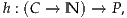 |
so the type of the recursion principle would be recC : ∏(P:) ((C →N) → P) → C → P,
and similarly for the induction principle. Now it is possible to write down a
computation rule, namely recC(P, h, g(α)) ≡ h(α). However, the existence
of a type C with this recursor and computation rule turns out to be
inconsistent. See Exercises 5.7 to 5.10 for proofs of this and other
variations.
This example suggests one restriction on inductive definitions: the
domains of all the constructors must be covariant functors of the type being
defined, so that we can “apply f to them” to get the result of the “recursive
call”. In other words, if we replace all occurrences of the type being defined
with a variable X : , then each domain of a constructor must be an
expression that can be made into a covariant functor of X. This is the case for
all the examples we have considered so far. For instance, with the constructor
inl : A → A + B, the relevant functor is constant at A (i.e. X A), while
for the constructor succ : N →N, the functor is the identity functor
(X
A), while
for the constructor succ : N →N, the functor is the identity functor
(X X).
X).
However, this necessary condition is also not sufficient. Covariance prevents the inductive type from occurring on the left of a single function type, as in the argument C →N of the “constructor” g considered above, since this yields a contravariant functor rather than a covariant one. However, since the composite of two contravariant functors is covariant, double function types such as ((X →N) →N) are once again covariant. This enables us to reproduce Cantorian-style paradoxes.
For instance, consider an “inductive type” D with the following constructor:
Assuming such a type exists, we define functions
| r | : D → (D →Prop) →Prop, | ||
| f | : (D →Prop) → D, | ||
| p | : (D →Prop) → (D →Prop) →Prop, | ||
| by | |||
| r(k(θ)) | :≡ θ, | ||
| f(δ) | :≡ k(λx.(x = δ)), | ||
| p(δ) | :≡ λx.δ(f(x)). | ||
In particular, therefore, if f(δ) = f(δ′), then we have a path s : (λx.(x = δ)) = (λx.(x = δ′)). Thus, happly(s, δ) : (δ = δ) = (δ = δ′), and so in particular δ = δ′ holds. Hence, f is “injective” (although a priori D may not be a set). This already sounds suspicious — we have an “injection” of the “power set” of D into D — and with a little more work we can massage it into a contradiction.
Suppose given θ : (D →Prop) →Prop, and define δ : D →Prop by
 | (5.6.2) |
We claim that p(δ) = θ. By function extensionality, it suffices to show p(δ)(γ) = Propθ(γ) for any γ : D →Prop. And by univalence, for this it suffices to show that each implies the other. Now by definition of p, we have
| p(δ)(γ) | ≡ δ(f(γ)) | ||
| ≡∃(γ′ : D →Prop).(f(γ′) = f(γ)) ×θ(γ′). |
This completes the proof that p(δ) = θ. Thus, every element θ : (D →Prop) →Prop is the image under p of some element δ : D →Prop. However, if we define θ by a classic diagonalization:

then from θ = p(δ) we deduce p(δ)(δ) = ¬p(δ)(δ). This is a contradiction: no proposition can be equivalent to its negation. (Supposing P ⇔¬P, if P, then ¬P, and so 0; hence ¬P, but then P, and so 0.)
Remark 5.6.3. There is a question of universe size to be addressed. In
general, an inductive type must live in a universe that already contains
all the types going into its definition. Thus if in the definition of D,
the ambiguous notation Prop means Prop, then we do not have D :
but only D : ′ for some larger universe ′ with : ′. In
a predicative theory, therefore, the right-hand side of (5.6.2) lives in
Prop′, not Prop. So this contradiction does require the propositional
resizing axiom mentioned in §3.5.
This counterexample suggests that we should ban an inductive type from ever appearing on the left of an arrow in the domain of its constructors, even if that appearance is nested in other arrows so as to eventually become covariant. (Similarly, we also forbid it from appearing in the domain of a dependent function type.) This restriction is called strict positivity (ordinary “positivity” being essentially covariance), and it turns out to suffice.
In conclusion, therefore, a valid inductive definition of a type W consists of a list of constructors. Each constructor is assigned a type that is a function type taking some number (possibly zero) of inputs (possibly dependent on one another) and returning an element of W. Finally, we allow W itself to occur in the input types of its constructors, but only strictly positively. This essentially means that each argument of a constructor is either a type not involving W, or some iterated function type with codomain W. For instance, the following is a valid constructor type:
 | (5.6.4) |
All of these function types can also be dependent functions (Π-types).1
Note we require that an inductive definition is given by a finite list of constructors. This is simply because we have to write it down on the page. If we want an inductive type which behaves as if it has an infinite number of constructors, we can simply parametrize one constructor by some infinite type. For instance, a constructor such as N → W → W can be thought of as equivalent to countably many constructors of the form W → W. (Of course, the infinity is now internal to the type theory, but this is as it should be for any foundational system.) Similarly, if we want a constructor that takes “infinitely many arguments”, we can allow it to take a family of arguments parametrized by some infinite type, such as (N → W) → W which takes an infinite sequence of elements of W.
Now, once we have such an inductive definition, what can we do with it? Firstly, there is a recursion principle stating that in order to define a function f : W → P, it suffices to consider the case when the input w : W arises from one of the constructors, allowing ourselves to recursively call f on the inputs to that constructor. For the example constructor (5.6.4), we would require P to be equipped with a function of type

 | (5.6.6) |
The induction principle for a general inductive type W is only a little
more complicated. Of course, we start with a type family P : W →, which
we require to be equipped with constructor data “lying over” the constructor
data of W. That means the “recursive call” arguments such as A → P above
must be replaced by dependent functions with types such as ∏(a:A) P(α(a)).
In the full example of (5.6.4), the corresponding hypothesis for the induction
principle would require
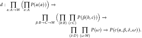 | (5.6.7) |
As discussed in §1.10, we also allow ourselves to invoke the induction and recursion principles implicitly, writing a definitional equation with :≡ for each expression that would be the hypotheses of the induction principle. This is called giving a definition by (dependent) pattern matching. In our running example, this means we could define f : ∏(w:W) P(w) by
where α : A → W and β : B → C → W and δ : D and ω : W are variables that are bound in the right-hand side. Moreover, the right-hand side may involve recursive calls to f of the form f(α(a)), f(β(b, c)), and f(ω). When this definition is repackaged in terms of the induction principle, we replace such recursive calls by (a), (b, c), and , respectively, for new variables
| : ∏ a:A P(α(a)) | |||
| : ∏ (b:B) ∏ (c:C) P(β(b, c)) | |||
| : P(ω). |

where the second argument to indW has the type of (5.6.7).
We will not attempt to give a formal presentation of the grammar of a valid inductive definition and its resulting induction and recursion principles and pattern matching rules. This is possible to do (indeed, it is necessary to do if implementing a computer proof assistant), but provides no additional insight. With practice, one learns to automatically deduce the induction and recursion principles for any inductive definition, and to use them without having to think twice.
The notion of inductive type has been studied in type theory for many years, and admits of many, many generalizations: inductive type families, mutual inductive types, inductive-inductive types, inductive-recursive types, etc. In this section we give an overview of some of these, a few of which will be used later in the book. (In Chapter 6 we will study in more depth a very different generalization of inductive types, which is particular to homotopy type theory.)
Most of these generalizations involve allowing ourselves to define more
than one type by induction at the same time. One very simple example of this,
which we have already seen, is the coproduct A + B. It would be tedious
indeed if we had to write down separate inductive definitions for N + N,
for N + 2, for 2 + 2, and so on every time we wanted to consider the
coproduct of two types. Instead, we make one definition in which A
and B are variables standing for types; in type theory they are called
parameters. Thus technically speaking, what results from the definition
is not a single type, but a family of types + : → →, taking
two types as input and producing their coproduct. Similarly, the type
List(A) of lists is a family List(–) : → in which the type A is a
parameter.
In mathematics, this sort of thing is so obvious as to not be worth
mentioning, but we bring it up in order to contrast it with the next example.
Note that each type A + B is independently defined inductively, as is each type
List(A). By contrast, we might also consider defining a whole type family
B : A → by induction together. The difference is that now the constructors
may change the index a : A, and as a consequence we cannot say that the
individual types B(a) are inductively defined, only that the entire family is
inductively defined.
The standard example is the type of lists of specified length, traditionally called vectors. We fix a parameter type A, and define a type family Vecn(A), for n : N, generated by the following constructors:
In contrast to lists, vectors (with elements from a fixed type A) form a family of types indexed by their length. While A is a parameter, we say that n : N is an index of the inductive family. An individual type such as Vec3(A) is not inductively defined: the constructors which build elements of Vec3(A) take input from a different type in the family, such as cons : A →Vec2(A) →Vec3(A).
In particular, the induction principle must refer to the entire type
family as well; thus the hypotheses and the conclusion must quantify
over the indices appropriately. In the case of vectors, the induction
principle states that given a type family C : ∏(n:N) Vecn(A) →, together
with
 |
there exists a function f : ∏(n:N) ∏(ℓ:Vecn(A)) C(n, ℓ) such that
| f(0, nil) | ≡ cnil | ||
| f(succ(n), cons(a, ℓ)) | ≡ ccons(n, a, ℓ, f(ℓ)). |
One use of inductive families is to define predicates inductively. For
instance, we might define the predicate iseven : N → as an inductive family
indexed by N, with the following constructors:
In other words, we stipulate that 0 is even, and that if n is even then so is succ(succ(n)). These constructors “obviously” give no way to construct an element of, say, iseven(1), and since iseven is supposed to be freely generated by these constructors, there must be no such element. (Actually proving that ¬iseven(1) is not entirely trivial, however). The induction principle for iseven says that to prove something about all even natural numbers, it suffices to prove it for 0 and verify that it is preserved by adding two.
Inductively defined predicates are much used in computer formalization of mathematics and software verification. But we will not have much use for them, with a couple of exceptions in §§10.3 and 11.5.
Another important special case is when the indexing type of an inductive family is finite. In this case, we can equivalently express the inductive definition as a finite collection of types defined by mutual induction. For instance, we might define the types even and odd of even and odd natural numbers by mutual induction, where even is generated by constructors
while odd is generated by the one constructor
Note that even and odd are simple types (not type families), but their constructors
can refer to each other. If we expressed this definition as an inductive type
family paritynat : 2 →, with paritynat(02) and paritynat(12) representing even
and odd respectively, it would instead have constructors:
When expressed explicitly as a mutual inductive definition, the induction
principle for even and odd says that given C : even → and D : odd →,
along with
there exist f : ∏(n:even) C(n) and g : ∏(n:odd) D(n) such that
| f(0) | ≡ c0 | ||
| f(esucc(n)) | ≡ cs(g(n)) | ||
| g(osucc(n)) | ≡ ds(f(n)). |
A further, more radical, generalization is to allow definition of a
type family B : A → in which not only the types B(a), but the type
A itself, is defined as part of one big induction. In other words, not
only do we specify constructors for the B(a)s which can take inputs
from other B(a′)s, as with inductive families, we also at the same time
specify constructors for A itself, which can take inputs from the B(a)s.
This can be regarded as an inductive family in which the indices are
inductively defined simultaneously with the indexed types, or as a
mutual inductive definition in which one of the types can depend on
the other. More complicated dependency structures are also possible.
In general, these are called inductive-inductive definitions. For the
most part, we will not use them in this book, but their higher variant
(see Chapter 6) will appear in a couple of experimental examples in
Chapter 11.
The last generalization we wish to mention is inductive-recursive definitions, in which a type is defined inductively at the same time as a recursive function on it. That is, we fix a known type P, and give constructors for an inductive type A and at the same time define a function f : A → P using the recursion principle for A resulting from its constructors — with the twist that the constructors of A are allowed to refer also to the values of f. We do not yet know how to justify such definitions from a homotopical perspective, and we will not use any of them in this book.
We now wish to point out that the identity types, which play so central a role in homotopy type theory, may also be considered to be defined inductively. Specifically, they are an “inductive family” with indices, in the sense of §5.7. In fact, there are two ways to describe identity types as an inductive family, resulting in the two induction principles described in Chapter 1, path induction and based path induction.
In both definitions, the type A is a parameter. For the first definition, we
inductively define a family = A : A → A →, with two indices belonging to
A, by the following constructor:
By analogy with the other inductive families, we may extract the induction principle from this definition. It states that given any
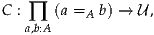 |
along with d : ∏(a:A) C(a, a, refla), there exists
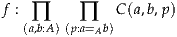 |
such that f(a, a, refla) ≡ d(a). This is exactly the path induction principle for identity types.
For the second definition, we consider one element a0 : A to be
a parameter along with A : , and we inductively define a family
(a0 = A–) : A →, with one index belonging to A, by the following
constructor:
Note that because a0 : A was fixed as a parameter, the constructor refla0 does
not appear inside the inductive definition as a function, but only an
element. The induction principle for this definition says that given
C : ∏(b:A) (a0 = Ab) → along with an element d : C(a0, refla0), there exists
f : ∏(b:A) ∏(p:a0=Ab) C(b, p) with f(a0, refla0) ≡ d. This is exactly the based
path induction principle for identity types.
The view of identity types as inductive types has historically caused some confusion, because of the intuition mentioned in §5.1 that all the elements of an inductive type should be obtained by repeatedly applying its constructors. For ordinary inductive types such as 2 and N, this is the case: we saw in Eq. (1.8.1) that indeed every element of 2 is either 02 or 12, and similarly one can prove that every element of N is either 0 or a successor.
However, this is not true for identity types: there is only one constructor
refl, but not every path is equal to the constant path. More precisely, we
cannot prove, using only the induction principle for identity types
(either one), that every inhabitant of a = Aa is equal to refla. In order to
actually exhibit a counterexample, we need some additional principle
such as the univalence axiom — recall that in Example 3.1.9 we used
univalence to exhibit a particular path 2 = 2 which is not equal to
refl2.
The point is that, as validated by the study of homotopy-initial algebras, an inductive definition should be regarded as freely generated by its constructors. Of course, a freely generated structure may contain elements other than its generators: for instance, the free group on two symbols x and y contains not only x and y but also words such as xy, yx-1y, and x3y2x-2yx. In general, the elements of a free structure are obtained by applying not only the generators, but also the operations of the ambient structure, such as the group operations if we are talking about free groups.
In the case of inductive types, we are talking about freely generated types — so what are the “operations” of the structure of a type? If types are viewed as like sets, as was traditionally the case in type theory, then there are no such operations, and hence we expect there to be no elements in an inductive type other than those resulting from its constructors. In homotopy type theory, we view types as like spaces or ∞-groupoids, in which case there are many operations on the paths (concatenation, inversion, etc.) — this will be important in Chapter 6 — but there are still no operations on the objects (elements). Thus, it is still true for us that, e.g., every element of 2 is either 02 or 12, and every element of N is either 0 or a successor.
However, as we saw in Chapter 2, viewing types as ∞-groupoids entails
also viewing functions as functors, and this includes type families B : A →.
Thus, the identity type (a0 = A–), viewed as an inductive type family, is
actually a freely generated functor A →. Specifically, it is the functor
F : A → freely generated by one element refla0 : F(a0). And a functor does
have operations on objects, namely the action of the morphisms (paths) of
A.
In category theory, the Yoneda lemma tells us that for any category A and object a0, the functor freely generated by an element of F(a0) is the representable functor hom A(a0, –). Thus, we should expect the identity type (a0 = A–) to be this representable functor, and this is indeed exactly how we view it: (a0 = Ab) is the space of morphisms (paths) in A from a0 to b.
One reason for viewing identity types as inductive families is to apply the uniqueness principles of §§5.2 and 5.5. Specifically, we can characterize the family of identity types of a type A, up to equivalence, by giving another family of types over A×A satisfying the same induction principle. This suggests the following definitions and theorem.
Definition 5.8.1. Let A be a type and a0 : A an element.
equipped
with an element r0 : R(a0).
and d : D(a0, r0), there exists
a function f : ∏(b:A) ∏(r:R(b)) D(b, r) such that f(a0, r0) = d.Note that the equivalences (i)⇔(ii)⇔(iii) are a version of Lemma 5.5.4 for identity types a0 = A–, regarded as inductive families varying over one element of A. Of course, (ii)–(iv) are mere propositions, so that logical equivalence implies actual equivalence. (Condition (i) is also a mere proposition, but we will not prove this.)
Proof. First, assume (i) and let (S, s0) be a pointed predicate. Define D(b, r) :≡ S(b) and d :≡ s0 : S(a0) ≡ D(a0, r0). Since R is an identity system, we have f : ∏(b:A) R(b) → S(b) with f(a0, r0) = s0; hence ppmap(R, S) is inhabited. Now suppose (f, fr), (g, gr) : ppmap(R, S), and define D(b, r) :≡ (f(b, r) = g(b, r)), and let d :≡ fr ▪ gr-1 : f(a0, r0) = s0 = g(a0, r0). Then again since R is an identity system, we have h : ∏(b:A) ∏(r:R(b)) D(b, r) such that h(a0, r0) = fr ▪gr-1. By the characterization of paths in Σ-types and path types, these data yield an equality (f, fr) = (g, gr). Hence ppmap(R, S) is an inhabited mere proposition, and thus contractible; so (ii) holds.
Now suppose (ii), and define S(b) :≡ (a0 = b) with s0 :≡ refla0 : S(a0). Then (S, s0) is a pointed predicate, and λb.λp.transportR(p, r) : ∏ (b:A) S(b) → R(b) is a pointed family of maps from S to R. By assumption, ppmap(R, S) is contractible, hence inhabited, so there also exists a pointed family of maps from R to S. And the composites in either direction are pointed families of maps from R to R and from S to S, respectively, hence equal to identities since ppmap(R, R) and ppmap(S, S) are contractible. Thus (iii) holds.
Now supposing (iii), condition (iv) follows from Lemma 3.11.8, using the fact that Σ-types respect equivalences (the “if” direction of Theorem 4.7.7).
Finally, assume (iv), and let D : ∏(b:A) R(b) → and d : D(a0, r0).
We can equivalently express D as a family D′ : ( ∑(b:A) R(b)) →. Now
since ∑(b:A) R(b) is contractible, we have
Moreover, since the path types of a contractible type are again contractible, we have p((a0, r0)) = refl(a0,r0). Define f(u) :≡ transportD′(p(u), d), yielding f : ∏(u:∑(b:A) R(b)) D′(u), or equivalently f : ∏(b:A) ∏(r:R(b)) D(b, r). Finally, we have
 " class="math-display" >
Thus, (i) holds. __
We can deduce a similar result for identity types = A, regarded as a family varying over two elements of A.
Definition 5.8.3. An identity system over a type A is a family R : A →
A → equipped with a function r0 : ∏(a:A) R(a, a) such that for any
type family D : ∏(a,b:A) R(a, b) → and d : ∏(a:A) D(a, a, r0(a)), there
exists a function f : ∏(a,b:A) ∏(r:R(b)) D(a, b, r) such that f(a, a, r0(a)) =
d(a) for all a : A.
Theorem 5.8.4. For R : A → A →equipped with r0 : ∏(a:A) R(a, a), the
following are logically equivalent.
and s0 : ∏(a:A) S(a, a), the type
Proof. The equivalence (i)⇔(ii) follows exactly the proof of equivalence between the path induction and based path induction principles for identity types; see §1.12. The equivalence with (iv) and (v) then follows from Theorem 5.8.2, while (iii) is straightforward. __
One reason this characterization is interesting is that it provides an
alternative way to state univalence and function extensionality. The
univalence axiom for a universe says exactly that the type family
together with id : ∏(A:) (A ≃ A) satisfies Theorem 5.8.4(iv). Therefore, it is
equivalent to the corresponding version of (i), which we can state as
follows.
Corollary 5.8.5 (Equivalence induction). Given any type family
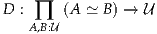 |
and function d : ∏(A:) D(A, A, idA), there exists
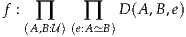 |
such that f(A, A, idA) = d(A) for all A : .
In other words, to prove something about all equivalences, it suffices to prove it about identity maps. We have already used this principle (without stating it in generality) in Lemma 4.1.1.
Similarly, function extensionality says that for any B : A →, the type
family
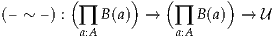
together with λf.λa.reflf(a) satisfies Theorem 5.8.4(iv). Thus, it is also equivalent to the corresponding version of (i).
Corollary 5.8.6 (Homotopy induction). Given any
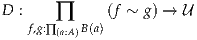 |
and d : ∏(f:∏(a:A) B(a)) D(f, f, λx.reflf(x)), there exists
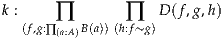 |
such that k(f, f, λx.reflf(x)) = d(f) for all f.
Inductive definitions have a long pedigree in mathematics, arguably going back at least to Frege and Peano’s axioms for the natural numbers. More general “inductive predicates” are not uncommon, but in set theoretic foundations they are usually constructed explicitly, either as an intersection of an appropriate class of subsets or using transfinite iteration along the ordinals, rather than regarded as a basic notion.
In type theory, particular cases of inductive definitions date back to Martin-Löf’s original papers: [ML71] presents a general notion of inductively defined predicates and relations; the notion of inductive type was present (but only with instances, not as a general notion) in Martin-Löf’s first papers in type theory [ML75]; and then as a general notion with W-types in [ML82].
A general notion of inductive type was introduced in 1985 by Constable and Mendler [CM85]. A general schema for inductive types in intensional type theory was suggested in [PPM90]. Further developments included [CP90, Dyb91].
The notion of inductive-recursive definition appears in [Dyb00]. An important type-theoretic notion is the notion of tree types (a general expression of the notion of Post system in type theory) which appears in [PS89].
The universal property of the natural numbers as an initial object of the category of N-algebras is due to Lawvere [Law06]. This was later generalized to a description of W-types as initial algebras for polynomial endofunctors by [MP00]. The coherently homotopy-theoretic equivalence between such universal properties and the corresponding induction principles (§§5.4 and 5.5) is due to [AGS12].
For actual constructions of inductive types in homotopy-theoretic semantics of type theory, see [KLV12, MvdB13, LS13b].
Exercise 5.1. Derive the induction principle for the type List(A) of lists from its definition as an inductive type in §5.1.
Exercise 5.2. Construct two functions on natural numbers which satisfy the same recurrence (ez, es) judgmentally, but are not judgmentally equal.
Exercise 5.3. Construct two different recurrences (ez, es) on the same type E which are both satisfied judgmentally by the same function f : N → E.
Exercise 5.5. Show that the analogous statement to Exercise 5.4 for N fails.
Exercise 5.6. Show that if we assume simple instead of dependent elimination for W-types, the uniqueness property (analogue of Theorem 5.3.1) fails to hold. That is, exhibit a type satisfying the recursion principle of a W-type, but for which functions are not determined uniquely by their recurrence.
Exercise 5.7. Suppose that in the “inductive definition” of the type C at the beginning of §5.6, we replace the type N by 0. Analogously to (5.6.1), we might consider a recursion principle for this type with hypothesis
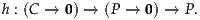
Show that even without a computation rule, this recursion principle is inconsistent, i.e. it allows us to construct an element of 0.
Exercise 5.8. Consider now an “inductive type” D with one constructor scott : (D → D) → D. The second recursor for C suggested in §5.6 leads to the following recursor for D:

with computation rule recD(P, h, scott(α)) ≡ h(α, (λd.recD(P, h, α(d)))). Show that this also leads to a contradiction.
Exercise 5.9. Let A be an arbitrary type and consider generally an “inductive definition” of a type LA with constructor lawvere : (LA → A) → LA. The second recursor for C suggested in §5.6 leads to the following recursor for LA:
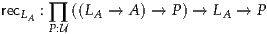
with computation rule recLA(P, h, lawvere(α)) ≡ h(α). Using this, show that A has the fixed-point property, i.e. for every function f : A → A there exists an a : A such that f(a) = a. In particular, LA is inconsistent if A is a type without the fixed-point property, such as 0, 2, or N.
Exercise 5.10. Continuing from Exercise 5.9, consider L1, which is not obviously inconsistent since 1 does have the fixed-point property. Formulate an induction principle for L1 and its computation rule, analogously to its recursor, and using this, prove that it is contractible.
Exercise 5.11. In §5.1 we defined the type List(A) of finite lists of elements of some type A. Consider a similar inductive definition of a type Lost(A) whose only constructor is

Show that Lost(A) is equivalent to 0.
Like the general inductive types we discussed in Chapter 5, higher inductive types are a general schema for defining new types generated by some constructors. But unlike ordinary inductive types, in defining a higher inductive type we may have “constructors” which generate not only points of that type, but also paths and higher paths in that type. For instance, we can consider the higher inductive type S1 generated by
This should be regarded as entirely analogous to the definition of, for instance, 2, as being generated by
or the definition of N as generated by
When we think of types as higher groupoids, the more general notion of “generation” is very natural: since a higher groupoid is a “multi-sorted object” with paths and higher paths as well as points, we should allow “generators” in all dimensions.
We will refer to the ordinary sort of constructors (such as base) as point constructors or ordinary constructors, and to the others (such as loop) as path constructors or higher constructors. Each path constructor must specify the starting and ending point of the path, which we call its source and target; for loop, both source and target are base.
Note that a path constructor such as loop generates a new inhabitant of an identity type, which is not (at least, not a priori) equal to any previously existing such inhabitant. In particular, loop is not a priori equal to reflbase (although proving that they are definitely unequal takes a little thought; see Lemma 6.4.1). This is what distinguishes S1 from the ordinary inductive type 1.
There are some important points to be made regarding this generalization.
First of all, the word “generation” should be taken seriously, in the same sense that a group can be freely generated by some set. In particular, because a higher groupoid comes with operations on paths and higher paths, when such an object is “generated” by certain constructors, the operations create more paths that do not come directly from the constructors themselves. For instance, in the higher inductive type S1, the constructor loop is not the only nontrivial path from base to base; we have also “loop ▪loop” and “loop ▪loop ▪loop” and so on, as well as loop-1, etc., all of which are different. This may seem so obvious as to be not worth mentioning, but it is a departure from the behavior of “ordinary” inductive types, where one can expect to see nothing in the inductive type except what was “put in” directly by the constructors.
Secondly, this generation is really free generation: higher inductive types do not technically allow us to impose “axioms”, such as forcing “loop ▪loop” to equal reflbase. However, in the world of ∞-groupoids, there is little difference between “free generation” and “presentation”, since we can make two paths equal up to homotopy by adding a new 2-dimensional generator relating them (e.g. a path loop ▪loop = reflbase in base = base). We do then, of course, have to worry about whether this new generator should satisfy its own “axioms”, and so on, but in principle any “presentation” can be transformed into a “free” one by making axioms into constructors. As we will see, by adding “truncation constructors” we can use higher inductive types to express classical notions such as group presentations as well.
Thirdly, even though a higher inductive type contains “constructors” which generate paths in that type, it is still an inductive definition of a single type. In particular, as we will see, it is the higher inductive type itself which is given a universal property (expressed, as usual, by an induction principle), and not its identity types. The identity type of a higher inductive type retains the usual induction principle of any identity type (i.e. path induction), and does not acquire any new induction principle.
Thus, it may be nontrivial to identify the identity types of a higher inductive type in a concrete way, in contrast to how in Chapter 2 we were able to give explicit descriptions of the behavior of identity types under all the traditional type forming operations. For instance, are there any paths from base to base in S1 which are not simply composites of copies of loop and its inverse? Intuitively, it seems that the answer should be no (and it is), but proving this is not trivial. Indeed, such questions bring us rapidly to problems such as calculating the homotopy groups of spheres, a long-standing problem in algebraic topology for which no simple formula is known. Homotopy type theory brings a new and powerful viewpoint to bear on such questions, but it also requires type theory to become as complex as the answers to these questions.
Fourthly, the “dimension” of the constructors (i.e. whether they output points, paths, paths between paths, etc.) does not have a direct connection to which dimensions the resulting type has nontrivial homotopy in. As a simple example, if an inductive type B has a constructor of type A → B, then any paths and higher paths in A result in paths and higher paths in B, even though the constructor is not a “higher” constructor at all. The same thing happens with higher constructors too: having a constructor of type A → (x =B y) means not only that points of A yield paths from x to y in B, but that paths in A yield paths between these paths, and so on. As we will see, this possibility is responsible for much of the power of higher inductive types.
On the other hand, it is even possible for constructors without higher types in their inputs to generate “unexpected” higher paths. For instance, in the 2-dimensional sphere S2 generated by
there is a nontrivial 3-dimensional path from reflreflbase to itself. Topologists will recognize this path as an incarnation of the Hopf fibration. From a category-theoretic point of view, this is the same sort of phenomenon as the fact mentioned above that S1 contains not only loop but also loop ▪loop and so on: it’s just that in a higher groupoid, there are operations which raise dimension. Indeed, we saw many of these operations back in §2.1: the associativity and unit laws are not just properties, but operations, whose inputs are 1-paths and whose outputs are 2-paths.
When we describe a higher inductive type such as the circle as being generated by certain constructors, we have to explain what this means by giving rules analogous to those for the basic type constructors from Chapter 1. The constructors themselves give the introduction rules, but it requires a bit more thought to explain the elimination rules, i.e. the induction and recursion principles. In this book we do not attempt to give a general formulation of what constitutes a “higher inductive definition” and how to extract the elimination rule from such a definition — indeed, this is a subtle question and the subject of current research. Instead we will rely on some general informal discussion and numerous examples.
The recursion principle is usually easy to describe: given any type equipped with the same structure with which the constructors equip the higher inductive type in question, there is a function which maps the constructors to that structure. For instance, in the case of S1, the recursion principle says that given any type B equipped with a point b : B and a path ℓ : b = b, there is a function f : S1 → B such that f(base) = b and apf(loop) = ℓ.
The latter two equalities are the computation rules. There is, however, a question of whether these computation rules are judgmental equalities or propositional equalities (paths). For ordinary inductive types, we had no qualms about making them judgmental, although we saw in Chapter 5 that making them propositional would still yield the same type up to equivalence. In the ordinary case, one may argue that the computation rules are really definitional equalities, in the intuitive sense described in the Introduction.
For higher inductive types, this is less clear. Moreover, since the operation apf is not really a fundamental part of the type theory, but something that we defined using the induction principle of identity types (and which we might have defined in some other, equivalent, way), it seems inappropriate to refer to it explicitly in a judgmental equality. Judgmental equalities are part of the deductive system, which should not depend on particular choices of definitions that we may make within that system. There are also semantic and implementation issues to consider; see the Notes.
It does seem unproblematic to make the computational rules for the point constructors of a higher inductive type judgmental. In the example above, this means we have f(base) ≡ b, judgmentally. This choice facilitates a computational view of higher inductive types. Moreover, it also greatly simplifies our lives, since otherwise the second computation rule apf(loop) = ℓ would not even be well-typed as a propositional equality; we would have to compose one side or the other with the specified identification of f(base) with b. (Such problems do arise eventually, of course, when we come to talk about paths of higher dimension, but that will not be of great concern to us here. See also §6.7.) Thus, we take the computation rules for point constructors to be judgmental, and those for paths and higher paths to be propositional.1
Remark 6.2.1. Recall that for ordinary inductive types, we regard the
computation rules for a recursively defined function as not merely
judgmental equalities, but definitional ones, and thus we may use the
notation :≡ for them. For instance, the truncated predecessor function
p : N →N is defined by p(0) :≡ 0 and p(succ(n)) :≡ n. In the case of
higher inductive types, this sort of notation is reasonable for the point
constructors (e.g. f(base) :≡ b), but for the path constructors it could
be misleading, since equalities such as f = ℓ are not judgmental.
Thus, we hybridize the notations, writing instead f
= ℓ are not judgmental.
Thus, we hybridize the notations, writing instead f : = ℓ for this
sort of “propositional equality by definition”.
: = ℓ for this
sort of “propositional equality by definition”.
Now, what about the induction principle (the dependent eliminator)? Recall that for an ordinary inductive type W, to prove by induction that ∏ (x:W) P(x), we must specify, for each constructor of W, an operation on P which acts on the “fibers” above that constructor in W. For instance, if W is the natural numbers N, then to prove by induction that ∏(x:N) P(x), we must specify
The second can be viewed as a function “P → P” lying over the constructor succ : N →N, generalizing how b : P(0) lies over the constructor 0 : N.
By analogy, therefore, to prove that ∏(x:S1) P(x), we should specify
Note that even though S1 contains paths other than loop (such as reflbase and loop ▪loop), we only need to specify a path lying over the constructor itself. This expresses the intuition that S1 is “freely generated” by its constructors.
The question, however, is what it means to have a path “lying over”
another path. It definitely does not mean simply a path b = b, since that would
be a path in the fiber P(base) (topologically, a path lying over the constant path
at base). Actually, however, we have already answered this question in
Chapter 2: in the discussion preceding Lemma 2.3.4 we concluded that a
path from u : P(x) to v : P(y) lying over p : x = y can be represented by a
path p* = v in the fiber P(y). Since we will have a lot of use for such
dependent paths in this chapter, we introduce a special notation for
them:
= v in the fiber P(y). Since we will have a lot of use for such
dependent paths in this chapter, we introduce a special notation for
them:
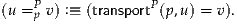 | (6.2.2) |
Remark 6.2.3. There are other possible ways to define dependent paths.
For instance, instead of p* = v we could consider u = (p-1)*
 . We
could also obtain it as a special case of a more general “heterogeneous
equality”, or with a direct definition as an inductive type family. All these
definitions result in equivalent types, so in that sense it doesn’t much
matter which we pick. However, choosing p*
. We
could also obtain it as a special case of a more general “heterogeneous
equality”, or with a direct definition as an inductive type family. All these
definitions result in equivalent types, so in that sense it doesn’t much
matter which we pick. However, choosing p* = v as the definition
makes it easiest to conclude other things about dependent paths, such
as the fact that apdf produces them, or that we can compute them in
particular type families using the transport lemmas in §2.5.
= v as the definition
makes it easiest to conclude other things about dependent paths, such
as the fact that apdf produces them, or that we can compute them in
particular type families using the transport lemmas in §2.5.
With the notion of dependent paths in hand, we can now state more
precisely the induction principle for S1: given P : S1 → and
there is a function f : ∏(x:S1) P(x) such that f(base) ≡ b and apdf = ℓ. As
in the non-dependent case, we speak of defining f by f(base) :≡ b and
apdf
= ℓ. As
in the non-dependent case, we speak of defining f by f(base) :≡ b and
apdf := ℓ.
:= ℓ.
Remark 6.2.4. When describing an application of this induction principle informally, we regard it as a splitting of the goal “P(x) for all x : S1” into two cases, which we will sometimes introduce with phrases such as “when x is base” and “when x varies along loop”, respectively. There is no specific mathematical meaning assigned to “varying along a path”: it is just a convenient way to indicate the beginning of the corresponding section of a proof; see Lemma 6.4.2 for an example.
Topologically, the induction principle for S1 can be visualized as
shown in Figure 6.1. Given a fibration over the circle (which in the
picture is a torus), to define a section of this fibration is the same as
to give a point b in the fiber over base along with a path from b to b
lying over loop. The way we interpret this type-theoretically, using our
definition of dependent paths, is shown in Figure 6.2: the path from b to b
over loop is represented by a path from loop* to b in the fiber over
base.
to b in the fiber over
base.
Of course, we expect to be able to prove the recursion principle from the induction principle, by taking P to be a constant type family. This is in fact the case, although deriving the non-dependent computation rule for loop (which refers to apf ) from the dependent one (which refers to apdf ) is surprisingly a little tricky.
Lemma 6.2.5. If Ais a type together with a : Aand p : a =A a, then there is a function f : S1 → Awith
| f(base) | :≡ a | ||
| apf(loop) | : = p. |
Proof. We would like to apply the induction principle of S1 to the
constant type family, (λx.A) : S1 →. The required hypotheses for this
are a point of (λx.A)(base) ≡ A, which we have (namely a : A), and a
dependent path in a =x Aloop a, or equivalently transportx
 A(loop, a) = a.
This latter type is not the same as the type a =A a where p lives, but it is
equivalent to it, because by Lemma 2.3.5 we have transportconstA loop(a) :
transportx
A(loop, a) = a.
This latter type is not the same as the type a =A a where p lives, but it is
equivalent to it, because by Lemma 2.3.5 we have transportconstA loop(a) :
transportx A(loop, a) = a. Thus, given a : A and p : a = a, we can
consider the composite
A(loop, a) = a. Thus, given a : A and p : a = a, we can
consider the composite

Applying the induction principle, we obtain f : S1 → A such that
| f(base) | ≡ a and | (6.2.6) |
| apdf(loop) | = transportconstA loop(a) ▪p. | (6.2.7) |

Combining this with (6.2.7) and canceling the occurrences of transportconst (which are the same by (6.2.6)), we obtain apf(loop) = p. __
We also have a corresponding uniqueness principle.
Lemma 6.2.8. If Ais a type and f, g : S1 → Aare two maps together with two equalities p, q:
| p : f(base) | = Ag(base), | ||
q : f | = pλx.x=Axg . . |
Proof. We apply the induction principle of S1 at the type family P(x) :≡
(f(x) = g(x)). When x is base, p is exactly what we need. And when x
varies along loop, we need  which by Theorems 2.11.3
and 2.11.5 can be reduced to q. __
which by Theorems 2.11.3
and 2.11.5 can be reduced to q. __
These two lemmas imply the expected universal property of the circle:
Proof. We have a canonical function f : (S1 → A) → ∑(x:A) (x = x)
defined by f(g) :≡ (g(base), g ). The induction principle shows
that the fibers of f are inhabited, while the uniqueness principle shows
that they are mere propositions. Hence they are contractible, so f is an
equivalence. __
). The induction principle shows
that the fibers of f are inhabited, while the uniqueness principle shows
that they are mere propositions. Hence they are contractible, so f is an
equivalence. __
As in §5.5, we can show that the conclusion of Lemma 6.2.9 is equivalent to having an induction principle with propositional computation rules. Other higher inductive types also satisfy lemmas analogous to Lemmas 6.2.5 and 6.2.9; we will generally leave their proofs to the reader. We now proceed to consider many examples.
The interval, which we denote I, is perhaps an even simpler higher inductive type than the circle. It is generated by:
The recursion principle for the interval says that given a type B along with
there is a function f : I → B such that f(0I) ≡ b0, f(1I) ≡ b1, and f = s. The
induction principle says that given P : I → along with
= s. The
induction principle says that given P : I → along with
there is a function f : ∏(x:I) P(x) such that f(0I) ≡ b0, f(1I) ≡ b1, and
apdf = s.
= s.
Regarded purely up to homotopy, the interval is not really interesting:
Proof. We prove that for all x : I we have x = I1I. In other words we want a function f of type ∏(x:I) (x = I1I). We begin to define f in the following way:
| f(0I) | :≡seg | : 0I | = I1I, | ||||
| f(1I) | :≡refl1I | : 1I | = I1I. |
 , which must have type seg = segλx.x=I1Irefl1
I .
By definition this type is seg*
, which must have type seg = segλx.x=I1Irefl1
I .
By definition this type is seg* = 1I=I1Irefl1I , which in turn is equivalent to
seg-1 ▪seg = refl1I . But there is a canonical element of that type, namely the
proof that path inverses are in fact inverses. __
= 1I=I1Irefl1I , which in turn is equivalent to
seg-1 ▪seg = refl1I . But there is a canonical element of that type, namely the
proof that path inverses are in fact inverses. __
However, type-theoretically the interval does still have some interesting features, just like the topological interval in classical homotopy theory. For instance, it enables us to give an easy proof of function extensionality. (Of course, as in §4.9, for the duration of the following proof we suspend our overall assumption of the function extensionality axiom.)
Lemma 6.3.2. If f, g : A → B are two functions such that f(x) = g(x) for every x : A, then f = g in the type A → B.
Proof. Let’s call the proof we have p : ∏(x:A) (f(x) = g(x)). For all x : A we
define a function  x : I → B by
 x(0I) x(0I) | :≡ f(x), | ||
 x(1I) x(1I) | :≡ g(x), | ||
 x x | : = p(x). |
Then q(0I) is the function λx. x(0I), which is equal to f because
  x(0I) is
defined by f(x). Similarly, we have q(1I) = g, and hence
x(0I) is
defined by f(x). Similarly, we have q(1I) = g, and hence
In Exercise 6.10 we ask the reader to complete the proof of the full function extensionality axiom from Lemma 6.3.2.
We have already discussed the circle S1 as the higher inductive type generated by
Its induction principle says that given P : S1 → along with b : P(base) and
ℓ : b =Ploop b, we have f : ∏(x:S1) P(x) with f(base) ≡ b and apdf = ℓ. Its
non-dependent recursion principle says that given B with b : B and ℓ : b = b,
we have f : S1 → B with f(base) ≡ b and f
= ℓ. Its
non-dependent recursion principle says that given B with b : B and ℓ : b = b,
we have f : S1 → B with f(base) ≡ b and f = ℓ.
= ℓ.
We observe that the circle is nontrivial.
Proof. Suppose that loop = reflbase. Then since for any type A with x : A
and p : x = x, there is a function f : S1 → A defined by f(base) :≡ x and
f : = p, we have

But this implies that every type is a set, which as we have seen is not the case (see Example 3.1.9). __
The circle also has the following interesting property, which is useful as a source of counterexamples.
Proof. We define f : ∏(x:S1) (x = x) by S1-induction. When x is base, we
let f(base) :≡ loop. Now when x varies along loop (see Remark 6.2.4),
we must show that transportx x=x(loop, loop) = loop. However, in §2.11
we observed that transportx
x=x(loop, loop) = loop. However, in §2.11
we observed that transportx x=x(p, q) = p-1 ▪q▪p, so what we have to
show is that loop-1 ▪loop ▪loop = loop. But this is clear by canceling an
inverse.
x=x(p, q) = p-1 ▪q▪p, so what we have to
show is that loop-1 ▪loop ▪loop = loop. But this is clear by canceling an
inverse.
To show that f≠(x reflx), it suffices to show that f(base)≠reflbase.
But f(base) = loop, so this is just the previous lemma. __
reflx), it suffices to show that f(base)≠reflbase.
But f(base) = loop, so this is just the previous lemma. __
For instance, this enables us to extend Example 3.1.9 by showing that any universe which contains the circle cannot be a 1-type.
Proof. The type S1 = S1 in is, by univalence, equivalent to the type
S1 ≃S1 of autoequivalences of S1, so it suffices to show that S1 ≃S1 is
not a set. For this, it suffices to show that its equality type idS1 =(S1≃S1)
id
S1 is not a mere proposition. Since being an equivalence is a mere
proposition, this type is equivalent to idS1 =(S1→S1) idS1. But by function
extensionality, this is equivalent to ∏(x:S1) (x = x), which as we have
seen in Lemma 6.4.2 contains two unequal elements. __
We have also mentioned that the 2-sphere S2 should be the higher inductive type generated by
The recursion principle for S2 is not hard: it says that given B with b : B and
s : reflb = reflb, we have f : S2 → B with f(base) ≡ b and ap2 f = s. Here
by “ap2 f
= s. Here
by “ap2 f ” we mean an extension of the functorial action of f to
two-dimensional paths, which can be stated precisely as follows.
” we mean an extension of the functorial action of f to
two-dimensional paths, which can be stated precisely as follows.
Lemma 6.4.4. Given f : A → B and x, y : Aand p, q : x = y, and r : p = q,
we have a path ap2 f : f
: f = f
= f .
.
Proof. By path induction, we may assume p ≡ q and r is reflexivity. But
then we may define ap2 f :≡reflf
 . __
. __
In order to state the general induction principle, we need a version of this lemma for dependent functions, which in turn requires a notion of dependent two-dimensional paths. As before, there are many ways to define such a thing; one is by way of a two-dimensional version of transport.
Lemma 6.4.5. Given P : A →and x, y : Aand p, q : x = yand r : p = q,
for any u : P(x) we have transport2 : p*
: p* = q*
= q* .
.
Proof. By path induction. __
Now suppose given x, y : A and p, q : x = y and r : p = q and also points
u : P(x) and v : P(y) and dependent paths h : u =Pp v and k : u =Pq v. By our
definition of dependent paths, this means h : p* = v and k : q*
 = v.
Thus, it is reasonable to define the type of dependent 2-paths over r to
be
= v.
Thus, it is reasonable to define the type of dependent 2-paths over r to
be

We can now state the dependent version of Lemma 6.4.4.
Lemma 6.4.6. Given P : A →and x, y : Aand p, q : x = yand r : p = q
and a function f : ∏(x:A) P(x), we have apd2 f : apdf
 =Pr apdf
 .
.
Proof. Path induction. __
Now we can state the induction principle for S2: given P : S2 → with
b : P(base) and s : reflb =Psurf reflb, there is a function f : ∏(x:S2) P(x) such that
f(base) ≡ b and apd2 f = s.
= s.
Of course, this explicit approach gets more and more complicated as we go up in dimension. Thus, if we want to define n-spheres for all n, we need some more systematic idea. One approach is to work with n-dimensional loops directly, rather than general n-dimensional paths.
Recall from §2.1 the definitions of pointed types *, and the n-fold
loop space Ωn : *→* (Definitions 2.1.7 and 2.1.8). Now we can
define the n-sphere Sn to be the higher inductive type generated by
In order to write down the induction principle for this presentation, we would need to define a notion of “dependent n-loop”, along with the action of dependent functions on n-loops. We leave this to the reader (see Exercise 6.4); in the next section we will discuss a different way to define the spheres that is sometimes more tractable.
The suspension of a type A is the universal way of making the points of A into paths (and hence the paths in A into 2-paths, and so on). It is a type ΣA defined by the following generators:2
The names are intended to suggest a “globe” of sorts, with a north pole, a south pole, and an A’s worth of meridians from one to the other. Indeed, as we will see, if A = S1, then its suspension is equivalent to the surface of an ordinary sphere, S2.
The recursion principle for ΣA says that given a type B together with
wehave a function f : ΣA → B such that f(N) ≡ n and f(S) ≡ s, and for all a : A
we have f = m(a). Similarly, the induction principle says that
given P : ΣA → together with
= m(a). Similarly, the induction principle says that
given P : ΣA → together with
there exists a function f : ∏(x:ΣA) P(x) such that f(N) ≡ n and f(S) ≡ s and for
each a : A we have apdf = m(a).
Our first observation about suspension is that it gives another way to define the circle.
Proof. Define f : Σ2 → S1 by recursion such that f(N) :≡ base and
f(S) :≡ base, while f : = loop but f
 : = reflbase.
Define g : S1 → Σ2 by recursion such that g(base) :≡N and g
: = reflbase.
Define g : S1 → Σ2 by recursion such that g(base) :≡N and g : =
merid(02) ▪merid(12)-1. We now show that f and g are quasi-inverses.
: =
merid(02) ▪merid(12)-1. We now show that f and g are quasi-inverses.
First we show by induction that g(f(x)) = x for all x : Σ2. If x ≡ N, then g(f(N)) ≡ g(base) ≡ N, so we have reflN : g(f(N)) = N. If x ≡ S, then g(f(S)) ≡ g(base) ≡ N, and we choose the equality merid(12) : g(f(S)) = S. It remains to show that for any y : 2, these equalities are preserved as x varies along merid(y), which is to say that when reflN is transported along merid(y) it yields merid(12). By transport in path spaces and pulled back fibrations, this means we are to show that

Of course, we may cancel reflN. Now by 2-induction, we may assume either y ≡ 02 or y ≡ 12. If y ≡ 02, then we have
g -1 ▪merid(0
2) -1 ▪merid(0
2) | = g -1 ▪merid(0
2) -1 ▪merid(0
2) | ||
| = (merid(02) ▪merid(12)-1)-1 ▪merid(0 2) | |||
| = merid(12) ▪merid(02)-1 ▪merid(0 2) | |||
| = merid(12) |
g -1 ▪merid(1
2) -1 ▪merid(1
2) | = g -1 ▪merid(1
2) -1 ▪merid(1
2) | ||
| = reflN-1 ▪merid(12) | |||
| = merid(12). |
Now we show by induction that f(g(x)) = x for all x : S1. If x ≡base, then f(g(base)) ≡ f(N) ≡base, so we have reflbase : f(g(base)) = base. It remains to show that this equality is preserved as x varies along loop, which is to say that it is transported along loop to itself. Again, by transport in path spaces and pulled back fibrations, this means to show that

However, we have
f | = f | ||
= f ▪f ▪f -1 -1 | |||
| = loop ▪reflbase |
Topologically, the two-point space 2 is also known as the 0-dimensional sphere, S0. (For instance, it is the space of points at distance 1 from the origin in R1, just as the topological 1-sphere is the space of points at distance 1 from the origin in R2.) Thus, Lemma 6.5.1 can be phrased suggestively as ΣS0 ≃S1. In fact, this pattern continues: we can define all the spheres inductively by
 | (6.5.2) |
We can even start one dimension lower by defining S-1 :≡0, and observe that Σ0 ≃2.
To prove carefully that this agrees with the definition of Sn from the previous section would require making the latter more explicit. However, we can show that the recursive definition has the same universal property that we would expect the other one to have. If (A, a0) and (B, b0) are pointed types (with basepoints often left implicit), let Map*(A, B) denote the type of based maps:
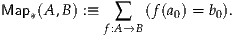
Note that any type A gives rise to a pointed type A+ :≡ A + 1 with basepoint inr(⋆); this is called adjoining a disjoint basepoint.
Note that on the right we have the ordinary type of unbased functions from A to B.
Proof. From left to right, given f : A+ → B with p : f(inr(⋆)) = b0, we have f ∘inl : A → B. And from right to left, given g : A → B we define g′ : A+ → B by g′(inl(a)) :≡ g(a) and g′(inr(u)) :≡ b0. We leave it to the reader to show that these are quasi-inverse operations. __
In particular, note that 2 ≃1+. Thus, for any pointed type B we have

Now recall that the loop space operation Ω acts on pointed types, with definition Ω(A, a0) :≡ (a0 =A a0, refla0). We can also make the suspension Σ act on pointed types, by Σ(A, a0) :≡ (ΣA, N).
Proof. We first observe the following chain of equivalences:
| Map*(ΣA, B) | :≡ ∑ f:ΣA→B (f(N) = b0) | ||
| ≃ ∑ f:∑(bn:B) ∑(bs:B)(A→(bn=bs)) (pr1(f) = b0) | |||
≃ ∑
(bn:B) ∑
(bs:B)  A → (bn = bs) A → (bn = bs) × (bn = b0) × (bn = b0) | |||
| ≃ ∑ (p:∑(bn:B)(bn=b0)) ∑ (bs:B) (A → (pr1(p) = bs)) | |||
| ≃ ∑ bs:B (A → (b0 = bs)) |
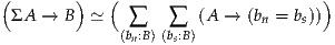
with the function from right to left given by the recursor (see Exercise 6.11). The second and third equivalences are by Exercise 2.10, along with a reordering of components. Finally, the last equivalence follows from Lemma 3.11.9, since by Lemma 3.11.8, ∑(bn:B) (bn = b0) is contractible with center (b0, reflb0).
The proof is now completed by the following chain of equivalences:
| ∑ bs:B (A → (b0 = bs)) | ≃ ∑ (bs:B) ∑ (g:A→(b0=bs)) ∑ (q:b0=bs) (g(a0) = q) | ||
| ≃ ∑ (r:∑(bs:B)(b0=bs)) ∑ (g:A→(b0=pr1(r))) (g(a0) = pr2(r)) | |||
| ≃ ∑ g:A→(b0=b0) (g(a0) = reflb0) | |||
| ≡Map*(A, ΩB). |
In particular, for the spheres defined as in (6.5.2) we have

Thus, these spheres Sn have the universal property that we would expect from the spheres defined directly in terms of n-fold loop spaces as in §6.4.
In classical topology, a cell complex is a space obtained by successively attaching discs along their boundaries. It is called a CW complex if the boundary of an n-dimensional disc is constrained to lie in the discs of dimension strictly less than n (the (n- 1)-skeleton).
Any finite CW complex can be presented as a higher inductive type, by turning n-dimensional discs into n-dimensional paths and partitioning the image of the attaching map into a source and a target, with each written as a composite of lower dimensional paths. Our explicit definitions of S1 and S2 in §6.4 had this form.
Another example is the torus T2, which is generated by:
Perhaps the easiest way to see that this is a torus is to start with a rectangle, having four corners a, b, c, d, four edges p, q, r, s, and an interior which is manifestly a 2-path t from p▪q to r▪s:
 |
Now identify the edge r with q and the edge s with p, resulting in also identifying all four corners. Topologically, this identification can be seen to produce a torus.
The induction principle for the torus is the trickiest of any we’ve
written out so far. Given P : T2 →, for a section ∏(x:T2) P(x) we
require
In order to make sense of this last datum, we need a composition operation for
dependent paths, but this is not hard to define. Then the induction principle
gives a function f : ∏(x:T2) P(x) such that f(b) ≡ b′ and apdf = p′ and
apdf
= p′ and
apdf = q′ and something like “apd2 f
 = t′”. However, this is not
well-typed as it stands, firstly because the equalities apdf
= t′”. However, this is not
well-typed as it stands, firstly because the equalities apdf = p′ and
apdf
= p′ and
apdf = q′ are not judgmental, and secondly because apdf only preserves
path concatenation up to homotopy. We leave the details to the reader (see
Exercise 6.1).
= q′ are not judgmental, and secondly because apdf only preserves
path concatenation up to homotopy. We leave the details to the reader (see
Exercise 6.1).
Of course, another definition of the torus is T2 :≡S1 ×S1 (in Exercise 6.3 we ask the reader to verify the equivalence of the two). The cell-complex definition, however, generalizes easily to other spaces without such descriptions, such as the Klein bottle, the projective plane, etc. But it does get increasingly difficult to write down the induction principles, requiring us to define notions of dependent n-paths and of apd acting on n-paths. Fortunately, once we have the spheres in hand, there is a way around this.
In topology, one usually speaks of building CW complexes by attaching n-dimensional discs along their (n- 1)-dimensional boundary spheres. However, another way to express this is by gluing in the cone on an (n- 1)-dimensional sphere. That is, we regard a disc as consisting of a cone point (or “hub”), with meridians (or “spokes”) connecting that point to every point on the boundary, continuously, as shown in Figure 6.3.
We can use this idea to express higher inductive types containing n-dimensional path-constructors for n > 1 in terms of ones containing only 1-dimensional path-constructors. The point is that we can obtain an n-dimensional path as a continuous family of 1-dimensional paths parametrized by an (n- 1)-dimensional object. The simplest (n- 1)-dimensional object to use is the (n- 1)-sphere, although in some cases a different one may be preferable. (Recall that we were able to define the spheres in §6.5 inductively using suspensions, which involve only 1-dimensional path constructors. Indeed, suspension can also be regarded as an instance of this idea, since it involves a family of 1-dimensional paths parametrized by the type being suspended.)
For instance, the torus T2 from the previous section could be defined instead to be generated by:
 : = p▪q▪p-1 ▪q-1.
The induction principle for this version of the torus says that given P : T2 →,
for a section ∏(x:T2) P(x) we require
 : = p′▪q′▪ (p′)-1 ▪ (q′)-1.
Note that there is no need for dependent 2-paths or apd2. We leave it to the reader to write out the computation rules.
Remark 6.7.1. One might question the need for introducing the hub point h; why couldn’t we instead simply add paths continuously relating the boundary of the disc to a point on that boundary, as shown in Figure 6.4? However, this does not work without further modification. For if, given some f : S1 → X, we give a path constructor connecting each f(x) to f(base), then what we end up with is more like the picture in Figure 6.5 of a cone whose vertex is twisted around and glued to some point on its base. The problem is that the specified path from f(base) to itself may not be reflexivity. We could remedy the problem by adding a 2-dimensional path constructor to ensure this, but using a separate hub avoids the need for any path constructors of dimension above 1.
Remark 6.7.2. Note also that this “translation” of higher paths into 1-paths does not preserve judgmental computation rules for these paths, though it does preserve propositional ones.
From a category-theoretic point of view, one of the important aspects of any foundational system is the ability to construct limits and colimits. In set-theoretic foundations, these are limits and colimits of sets, whereas in our case they are limits and colimits of types. We have seen in §2.15 that cartesian product types have the correct universal property of a categorical product of types, and in Exercise 2.9 that coproduct types likewise have their expected universal property.
As remarked in §2.15, more general limits can be constructed using identity types and Σ-types, e.g. the pullback of f : A → C and g : B → C is ∑ (a:A) ∑(b:B) (f(a) = g(b)) (see Exercise 2.11). However, more general colimits require identifying elements coming from different types, for which higher inductives are well-adapted. Since all our constructions are homotopy-invariant, all our colimits are necessarily homotopy colimits, but we drop the ubiquitous adjective in the interests of concision.
In this section we discuss pushouts, as perhaps the simplest and one of the most useful colimits. Indeed, one expects all finite colimits (for a suitable homotopical definition of “finite”) to be constructible from pushouts and finite coproducts. It is also possible to give a direct construction of more general colimits using higher inductive types, but this is somewhat technical, and also not completely satisfactory since we do not yet have a good fully general notion of homotopy coherent diagrams.
Suppose given a span of types and functions:
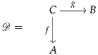
The pushout of this span is the higher inductive type A⊔CB presented by
In other words, A⊔CB is the disjoint union of A and B, together with for every c : C a witness that f(c) and g(c) are equal. The recursion principle says that if D is another type, we can define a map s : A⊔CB → D by defining
We leave it to the reader to formulate the induction principle. It also implies the uniqueness principle that if s, s′ : A⊔CB → D are two maps such that
| s(inl(a)) | = s′(inl(a)) | ||
| s(inr(b)) | = s′(inr(b)) | ||
| aps(glue(c)) | = aps′(glue(c)) (modulo the previous two equalities) |
To formulate the universal property of a pushout, we introduce the following.
Definition 6.8.1. Given a span  = (A
= (A
 ) and a type D, a cocone
under with vertex D consists of functions i : A → D and j : B → D
and a homotopy h : ∏(c:C) (i(f(c)) = j(g(c))):
) and a type D, a cocone
under with vertex D consists of functions i : A → D and j : B → D
and a homotopy h : ∏(c:C) (i(f(c)) = j(g(c))):

We denote by cocone (D) the type of all such cocones, i.e.

Of course, there is a canonical cocone under with vertex A⊔CB
consisting of inl, inr, and glue.
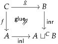
The following lemma says that this is the universal such cocone.
Proof. Let’s consider an arbitrary type E : . There is a canonical function
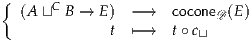
defined by sending (i, j, h) to (t∘i, t∘j, apt ∘h). We show that this is an equivalence.
Firstly, given a c = (i, j, h) : cocone (E), we need to construct a map
s(c) from A⊔CB to E.

The map s(c) is defined in the following way
| s(c)(inl(a)) | :≡ i(a), | ||
| s(c)(inr(b)) | :≡ j(b), | ||
| aps(c)(glue(x)) | : = h(x). |
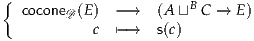
and we need to prove that this map is an inverse to t t∘c⊔. On the one
hand, if c = (i, j, h) : cocone (E), we have
t∘c⊔. On the one
hand, if c = (i, j, h) : cocone (E), we have
| s(c) ∘c⊔ | = (s(c) ∘inl, s(c) ∘inr, aps(c) ∘glue) | ||
| = (λa.s(c)(inl(a)), λb.s(c)(inr(b)), λx.aps(c)(glue(x))) | |||
| = (λa.i(a), λb.j(b), λx.h(x)) | |||
| ≡ (i, j, h) | |||
| = c. |
because the first component of t∘c⊔ is t∘inl. In the same way, for b : B we have
and for x : C we have
hence s(t∘c⊔) = t.
This proves that c s(c) is a quasi-inverse to t
 t∘c⊔, as desired. __
A number of standard homotopy-theoretic constructions can be expressed as (homotopy) pushouts.
 ×B
×B is called the join of A and B, written
A*B.
is called the join of A and B, written
A*B.
 is the cone or cofiber of f.

 is the wedge A∨B.
 : =
refl
(a0,b0). Then the cone of f is called the smash product A∧B.
: =
refl
(a0,b0). Then the cone of f is called the smash product A∧B.We will discuss pushouts further in Chapters 7 and 8.
Remark 6.8.3. As remarked in §3.7, the notations ∧ and ∨ for the smash product and wedge of pointed spaces are also used in logic for “and” and “or”, respectively. Since types in homotopy type theory can behave either like spaces or like propositions, there is technically a potential for conflict — but since they rarely do both at once, context generally disambiguates. Furthermore, the smash product and wedge only apply to pointed spaces, while the only pointed mere proposition is ⊤≡1 — and we have 1 ∧1 = 1 and 1 ∨1 = 1 for either meaning of ∧ and ∨.
Remark 6.8.4. Note that colimits do not in general preserve truncatedness. For instance, S0 and 1 are both sets, but the pushout of 1 ←S0 →1 is S1, which is not a set. If we are interested in colimits in the category of n-types, therefore (and, in particular, in the category of sets), we need to “truncate” the colimit somehow. We will return to this point in §6.9 and Chapters 7 and 10.
In §3.7 we introduced the propositional truncation as a new type forming operation; we now observe that it can be obtained as a special case of higher inductive types. This reduces the problem of understanding truncations to the problem of understanding higher inductives, which at least are amenable to a systematic treatment. It is also interesting because it provides our first example of a higher inductive type which is truly recursive, in that its constructors take inputs from the type being defined (as does the successor succ : N →N).
Let A be a type; we define its propositional truncation  to be the
higher inductive type generated by:
to be the
higher inductive type generated by:
 , and
, and
 , a path x = y.
Note that the second constructor is by definition the assertion that  is a mere
proposition. Thus, the definition of
is a mere
proposition. Thus, the definition of  can be interpreted as saying that
 is freely generated by a function A →
 and the fact that it is a mere
proposition.
and the fact that it is a mere
proposition.
The recursion principle for this higher inductive definition is easy to write down: it says that given any type B together with
there exists a function f :  → B such that
 ) ≡ g(a) for all a : A, and
 , the function apf takes the specified path x = y
in
, the function apf takes the specified path x = y
in  to the specified path f(x) = f(y) in B (propositionally).
These are exactly the hypotheses that we stated in §3.7 for the recursion principle of propositional truncation — a function A → B such that B is a mere proposition — and the first part of the conclusion is exactly what we stated there as well. The second part (the action of apf ) was not mentioned previously, but it turns out to be vacuous in this case, because B is a mere proposition, so any two paths in it are automatically equal.
There is also an induction principle for  , which says that given any
B :
, which says that given any
B :  → together with
 ), and
 and u : B(x) and v : B(y), a dependent path
q : u =Bp(x,y) v, where p(x, y) is the path coming from the second
constructor of
and u : B(x) and v : B(y), a dependent path
q : u =Bp(x,y) v, where p(x, y) is the path coming from the second
constructor of  ,
,there exists f : ∏(x:∥A∥) B(x) such that f( ) ≡ g(a) for a : A, and also another
computation rule. However, because there can be at most one function
between any two mere propositions (up to homotopy), this induction
principle is not really useful (see also Exercise 3.17).
) ≡ g(a) for a : A, and also another
computation rule. However, because there can be at most one function
between any two mere propositions (up to homotopy), this induction
principle is not really useful (see also Exercise 3.17).
We can, however, extend this idea to construct similar truncations landing
in n-types, for any n. For instance, we might define the 0-truncation  0 to
be generated by
0 to
be generated by
 0, and
 0 and each p, q : x = y, a path p = q.
Then  0 would be freely generated by a function A →
 0 together with
the assertion that
0 together with
the assertion that  0 is a set. A natural induction principle for it would say
that given B :
0 is a set. A natural induction principle for it would say
that given B :  0 → together with
 0), and
 0 with z : B(x) and w : B(y), and each p, q : x = y
with r : z =Bp w and s : z =Bq w, a 2-path v : r =z=B-w
u(x,y,p,q) s,
where u(x, y, p, q) : p = q is obtained from the second constructor
of
0 with z : B(x) and w : B(y), and each p, q : x = y
with r : z =Bp w and s : z =Bq w, a 2-path v : r =z=B-w
u(x,y,p,q) s,
where u(x, y, p, q) : p = q is obtained from the second constructor
of  0,
0,there exists f : ∏(x:∥A∥
0) B(x) such that f( 0) ≡ g(a) for all a : A, and also
apd2
f
0) ≡ g(a) for all a : A, and also
apd2
f is the 2-path specified above. (As in the propositional case,
the latter condition turns out to be uninteresting.) From this, however, we can
prove a more useful induction principle.
is the 2-path specified above. (As in the propositional case,
the latter condition turns out to be uninteresting.) From this, however, we can
prove a more useful induction principle.
Lemma 6.9.1. Suppose given B :  0 → together with g :
∏
(a:A) B(
0 → together with g :
∏
(a:A) B( 0), and assume that each B(x) is a set. Then there exists f :
∏
(x:∥A∥0) B(x) such that f(
0), and assume that each B(x) is a set. Then there exists f :
∏
(x:∥A∥0) B(x) such that f( 0) ≡ g(a) for all a : A.
Proof. It suffices to construct, for any x, y, z, w, p, q, r, s as above, a 2-path v : r =Bu(x,y,p,q) s. However, by the definition of dependent 2-paths, this is an ordinary 2-path in the fiber B(y). Since B(y) is a set, a 2-path exists between any two parallel paths. __
This implies the expected universal property.
Proof. The special case of Lemma 6.9.1 when B is the constant family
gives a map from right to left, which is a right inverse to the “compose
with |–|0” function from left to right. To show that it is also a left inverse,
let h :  0 → B, and define h′ :
  0 → B by applying Lemma 6.9.1
to the composite a
0 → B by applying Lemma 6.9.1
to the composite a h(
h( 0). Thus, h′(
 0) = h(
 0).
0).
However, since B is a set, for any x :  0 the type h(x) = h′(x) is
a mere proposition, and hence also a set. Therefore, by Lemma 6.9.1, the
observation that h′(
0 the type h(x) = h′(x) is
a mere proposition, and hence also a set. Therefore, by Lemma 6.9.1, the
observation that h′( 0) = h(
 0) for any a : A implies h(x) = h′(x)
for any x :
0) for any a : A implies h(x) = h′(x)
for any x :  0, and hence h = h′. __
For instance, this enables us to construct colimits of sets. We have seen
that if A
 is a span of sets, then the pushout A⊔CB may no
longer be a set. (For instance, if A and B are 1 and C is 2, then the
pushout is S1.) However, we can construct a pushout that is a set,
and has the expected universal property with respect to other sets, by
truncating.
is a span of sets, then the pushout A⊔CB may no
longer be a set. (For instance, if A and B are 1 and C is 2, then the
pushout is S1.) However, we can construct a pushout that is a set,
and has the expected universal property with respect to other sets, by
truncating.
We refer to  0 as the set-pushout of f and g, to distinguish it
from the (homotopy) pushout A⊔CB. Alternatively, we could modify the
definition of the pushout in §6.8 to include the 0-truncation constructor
directly, avoiding the need to truncate afterwards. Similar remarks apply to
any sort of colimit of sets; we will explore this further in Chapter 10.
0 as the set-pushout of f and g, to distinguish it
from the (homotopy) pushout A⊔CB. Alternatively, we could modify the
definition of the pushout in §6.8 to include the 0-truncation constructor
directly, avoiding the need to truncate afterwards. Similar remarks apply to
any sort of colimit of sets; we will explore this further in Chapter 10.
However, while the above definition of the 0-truncation works — it gives
what we want, and is consistent — it has a couple of issues. Firstly, it doesn’t
fit so nicely into the general theory of higher inductive types. In general, it is
tricky to deal directly with constructors such as the second one we have given
for  0, whose inputs involve not only elements of the type being defined,
but paths in it.
0, whose inputs involve not only elements of the type being defined,
but paths in it.
This can be gotten round fairly easily, however. Recall in §5.1 we mentioned that we can allow a constructor of an inductive type W to take “infinitely many arguments” of type W by having it take a single argument of type N → W. There is a general principle behind this: to model a constructor with funny-looking inputs, use an auxiliary inductive type (such as N) to parametrize them, reducing the input to a simple function with inductive domain.
For the 0-truncation, we can consider the auxiliary higher inductive
type S generated by two points a, b : S and two paths p, q : a = b.
Then the fishy-looking constructor of  0 can be replaced by the
unobjectionable
0 can be replaced by the
unobjectionable
Since to give a map out of S is the same as to give two points and two parallel paths between them, this yields the same induction principle.
A more serious problem with our current definition of 0-truncation, however, is that it doesn’t generalize very well. If we want to describe a notion of definition of “n-truncation” into n-types uniformly for all n : N, then this approach is unfeasible, since the second constructor would need a number of arguments that increases with n. In §7.3, therefore, we will use a different idea to construct these, based on the observation that the type S introduced above is equivalent to the circle S1. This includes the 0-truncation as a special case, and satisfies generalized versions of Lemmas 6.9.1 and 6.9.2.
A particularly important sort of colimit of sets is the quotient by a relation. That is, let A be a set and R : A×A →Prop a family of mere propositions (a mere relation). Its quotient should be the set-coequalizer of the two projections
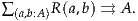
We can also describe this directly, as the higher inductive type A/R generated by
We will sometimes refer to this higher inductive type A/R as the set-quotient of A by R, to emphasize that it produces a set by definition. (There are more general notions of “quotient” in homotopy theory, but they are mostly beyond the scope of this book. However, in §9.9 we will consider the “quotient” of a type by a 1-groupoid, which is the next level up from set-quotients.)
Remark 6.10.1. It is not actually necessary for the definition of set-quotients, and most of their properties, that A be a set. However, this is generally the case of most interest.
Proof. We must show that for any x : A/R there merely exists an a : A with q(a) = x. We use the induction principle of A/R. The first case is trivial: if x is q(a), then of course there merely exists an a such that q(a) = q(a). And since the goal is a mere proposition, it automatically respects all path constructors, so we are done. __
We can now prove that the set-quotient has the expected universal property of a (set-)coequalizer.
Proof. The quasi-inverse of – ∘q, going from right to left, is just the recursion principle for A/R. That is, given f : A → B such that
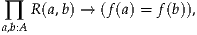 |
we define : A/R → B by (q(a)) :≡ f(a). This defining equation says
precisely that (f ) is a right inverse to (– ∘q).
For it to also be a left inverse, we must show that for any g : A/R → B and x : A/R we have g(x) = g∘q. However, by Lemma 6.10.2 there merely exists a such that q(a) = x. Since our desired equality is a mere proposition, we may assume there purely exists such an a, in which case g(x) = g(q(a)) = g∘q(q(a)) = g∘q(x). __
Of course, classically the usual case to consider is when R is an equivalence relation, i.e. we have
In this case, the set-quotient A/R has additional good properties, as we will see in §10.1: for instance, we have R(a, b) ≃ (q(a) =A/R q(b)). We often write an equivalence relation R(a, b) infix as a ~ b.
The quotient by an equivalence relation can also be constructed in other ways. The set theoretic approach is to consider the set of equivalence classes, as a subset of the power set of A. We can mimic this “impredicative” construction in type theory as well.
Definition 6.10.4. A predicate P : A →Prop is an equivalence class of a relation R : A×A →Prop if there merely exists an a : A such that for all b : A we have R(a, b) ≃ P(b).
As R and P are mere propositions, the equivalence R(a, b) ≃ P(b) is the same thing as implications R(a, b) → P(b) and P(b) → R(a, b). And of course, for any a : A we have the canonical equivalence class Pa(b) :≡ R(a, b).
Theorem 6.10.6. For any equivalence relation R on A, the type A ⫽// R is equivalent to the set-quotient A/R.
Proof. First, note that if R(a, b), then since R is an equivalence relation we have R(a, c) ⇔ R(b, c) for any c : A. Thus, R(a, c) = R(b, c) by univalence, hence Pa = Pb by function extensionality, i.e. q′(a) = q′(b). Therefore, by Lemma 6.10.3 we have an induced map f : A/R → A⫽//R such that f ∘q = q′.
We show that f is injective and surjective, hence an equivalence. Surjectivity follows immediately from the fact that q′ is surjective, which in turn is true essentially by definition of A⫽//R. For injectivity, if f(x) = f(y), then to show the mere proposition x = y, by surjectivity of q we may assume x = q(a) and y = q(b) for some a, b : A. Then R(a, c) = f(q(a))(c) = f(q(b))(c) = R(b, c) for any c : A, and in particular R(a, b) = R(b, b). But R(b, b) is inhabited, since R is an equivalence relation, hence so is R(a, b). Thus q(a) = q(b) and so x = y. __
In §10.1.3 we will give an alternative proof of this theorem. Note that
unlike A/R, the construction A⫽//R raises universe level: if A : i and
R : A → A →Propi, then in the definition of A⫽//R we must also use Propi
to include all the equivalence classes, so that A⫽//R : i+1. Of course, we
can avoid this if we assume the propositional resizing axiom from
§3.5.
Remark 6.10.7. The previous two constructions provide quotients in generality, but in particular cases there may be easier constructions. For instance, we may define the integers Z as a set-quotient
where ~ is the equivalence relation defined by

In other words, a pair (a, b) represents the integer a-b. In this case, however, there are canonical representatives of the equivalence classes: those of the form (n, 0) or (0, n).
The following lemma says that when this sort of thing happens, we don’t need either general construction of quotients. (A function r : A → A is called idempotent if r∘r = r.)
Lemma 6.10.8. Suppose ~is a relation on a set A, and there exists an idempotent r : A → Asuch that (r(x) = r(y)) ≃ (x ~ y) for all x, y : A. (This implies ~is an equivalence relation.) Then the type
 |
satisfies the universal property of the set-quotient of Aby ~, and hence is equivalent to it. In other words, there is a map q : A → (A/~) such that for every set B, precomposition with qinduces an equivalence
 | (6.10.9) |
Proof. Let i : ∏(x:A) r(r(x)) = r(x) witness idempotence of r. The map q : A → (A/~) is defined by q(x) :≡ (r(x), i(x)). Note that since A is a set, we have q(x) = q(y) if and only if r(x) = r(y), hence (by assumption) if and only if x ~ y. We define a map e from left to right in (6.10.9) by
where the underscore denotes the following proof: if x, y : A and x ~ y, then q(x) = q(y) as observed above, hence f(q(x)) = f(q(y)). To see that e is an equivalence, consider the map e′ in the opposite direction defined by
Given any f : (A/~) → B,

where the last equality holds because p : r(x) = x and so (x, p) = (r(x), i(x)) because A is a set. Similarly we compute

Because B is a set we need not worry about the part, while for the first component we have

where the last equation holds because r(x) ~ x, and g respects ~ by the assumption s. __
Corollary 6.10.10. Suppose p : A → B is a retraction between sets. Then B is the quotient of Aby the equivalence relation ~defined by
Proof. Suppose s : B → A is a section of p. Then s∘p : A → A is an idempotent which satisfies the condition of Lemma 6.10.8 for this ~, and s induces an isomorphism from B to its set of fixed points. __
Remark 6.10.11. Lemma 6.10.8 applies to Z with the idempotent r : N ×N →N ×N defined by
 |
(This is a valid definition even constructively, since the relation ≥ on N is decidable.) Thus a non-negative integer is canonically represented as (k, 0) and a non-positive one by (0, m), for k, m : N. This division into cases implies the following “induction principle” for integers, which will be useful in Chapter 8. (As usual, we identify a natural number n with the corresponding non-negative integer, i.e. with the image of (n, 0) : N ×N in Z.)
Lemma 6.10.12. Suppose P : Z →is a type family and that we have
Then we have f : ∏(z:Z) P(z) such that
Proof. For purposes of this proof, let Z denote ∑(x:N×N) (r(x) = x),
where r is the above idempotent. (We can then transport the result to
any equivalent definition of Z.) Let q : N ×N →Z be the quotient
map, defined by q(x) = (r(x), i(x)) as in Lemma 6.10.8. Now define
Q :≡ P ∘q : N ×N →. By transporting the given data across appropriate
equalities, we obtain
| d′0 | : Q(0, 0) | ||
| d′+ | : ∏ n:N Q(n, 0) → Q(succ(n), 0) | ||
| d′- | : ∏ n:N Q(0, n) → Q(0, succ(n)). |

We can then construct g : ∏(x:N×N) Q(x) by double induction on x:
| g(0, 0) | :≡ d′0, | ||
| g(succ(n), 0) | :≡ d′+(n, g(n, 0)), | ||
| g(0, succ(m)) | :≡ d′-(m, g(0, m)), | ||
| g(succ(n), succ(m)) | :≡ en,m(g(n, m)). |
We will sometimes denote a function f : ∏(z:Z) P(z) obtained from Lemma 6.10.12 with a pattern-matching syntax, involving the three cases d0, d+, and d-:
| f(0) | : = d0 | ||
| f(succ(n)) | : = d+(n, f(n)) | ||
| f(-succ(n)) | : = d-(n, f(-n)) |
Corollary 6.10.13. Let Abe a type with a : Aand p : a = a. There is a function
∏
(n:Z) (a = a), denoted n pn, defined by
| p0 | : = refla | ||||||
| pn+1 | : = pn ▪p | for n ≥ 0 | |||||
| pn-1 | : = pn ▪p-1 | for n ≤ 0. |
We will discuss the integers further in §§6.11 and 11.1.
In addition to constructing higher-dimensional objects such as spheres and cell complexes, higher inductive types are also very useful even when working only with sets. We have seen one example already in Lemma 6.9.3: they allow us to construct the colimit of any diagram of sets, which is not possible in the base type theory of Chapter 1. Higher inductive types are also very useful when we study sets with algebraic structure.
As a running example in this section, we consider groups, which are familiar to most mathematicians and exhibit the essential phenomena (and will be needed in later chapters). However, most of what we say applies equally well to any sort of algebraic structure.
Remark 6.11.2. Note that we require a group to be a set. We could consider a more general notion of “∞-group” which is not a set, but this would take us further afield than is appropriate at the moment. With our current definition, we may expect the resulting “group theory” to behave similarly to the way it does in set-theoretic mathematics (with the caveat that, unless we assume LEM, it will be “constructive” group theory).
Example 6.11.3. The natural numbers N are a monoid under addition, with unit 0, and also under multiplication, with unit 1. If we define the arithmetical operations on the integers Z in the obvious way, then as usual they are a group under addition and a monoid under multiplication (and, of course, a ring). For instance, if u, v ∈ Z are represented by (a, b) and (c, d), respectively, then u + v is represented by (a + c, b + d), -u is represented by (b, a), and uv is represented by (ac + bd, ad + bc).
Example 6.11.4. We essentially observed in §2.1 that if (A, a) is a pointed type, then its loop space Ω(A, a) :≡ (a =A a) has all the structure of a group, except that it is not in general a set. It should be an “∞-group” in the sense mentioned in Remark 6.11.2, but we can also make it a group by truncation. Specifically, we define the fundamental group of A based at a : A to be
This inherits a group structure; for instance, the multiplication π1(A, a) × π1(A, a) → π1(A, a) is defined by double induction on truncation from the concatenation of paths.
More generally, the nth homotopy group of (A, a) is πn(A, a) :≡
 0. Then πn(A, a) = π1(Ωn-1(A, a)) for n ≥ 1, so it is also a
group. (When n = 0, we have π0(A) ≡
0. Then πn(A, a) = π1(Ωn-1(A, a)) for n ≥ 1, so it is also a
group. (When n = 0, we have π0(A) ≡  0, which is not a group.)
Moreover, the Eckmann–Hilton argument (Theorem 2.1.6) implies that
if n ≥ 2, then πn(A, a) is an abelian group, i.e. we have x⋅y = y⋅x for
all x, y. Chapter 8 will be largely the study of these groups.
0, which is not a group.)
Moreover, the Eckmann–Hilton argument (Theorem 2.1.6) implies that
if n ≥ 2, then πn(A, a) is an abelian group, i.e. we have x⋅y = y⋅x for
all x, y. Chapter 8 will be largely the study of these groups.
One important notion in group theory is that of the free group generated by a set, or more generally of a group presented by generators and relations. It is well-known in type theory that some free algebraic objects can be defined using ordinary inductive types. For instance, the free monoid on a set A can be identified with the type List(A) of finite lists of elements of A, which is inductively generated by
We have an obvious inclusion η : A →List(A) defined by a cons(a, nil). The
monoid operation on List(A) is concatenation, defined recursively
by
cons(a, nil). The
monoid operation on List(A) is concatenation, defined recursively
by
| nil ⋅ℓ | :≡ ℓ | ||
| cons(a, ℓ1) ⋅ℓ2 | :≡cons(a, ℓ1 ⋅ℓ2). |
Lemma 6.11.5. For any set A, the type List(A) is the free monoid on A. In other words, for any monoid G, composition with η is an equivalence

where hom Monoid(–, –) denotes the set of monoid homomorphisms (functions which preserve the multiplication and unit).
Proof. Given f : A → G, we define : List(A) → G by recursion:
| (nil) | :≡ e | ||
| (cons(a, ℓ)) | :≡ f(a) ⋅(ℓ). |
 is a quasi-inverse of (– ∘η); see Exercise 6.8. __
This construction of the free monoid is possible essentially because elements of the free monoid have computable canonical forms (namely, finite lists). However, elements of other free (and presented) algebraic structures — such as groups — do not in general have computable canonical forms. For instance, equality of words in group presentations is algorithmically undecidable. However, we can still describe free algebraic objects as higher inductive types, by simply asserting all the axiomatic equations as path constructors.
For example, let A be a set, and define a higher inductive type F(A) with the following generators.
The first constructor says that A maps to F(A). The next three give F(A) the operations of a group: multiplication, an identity element, and inversion. The three constructors after that assert the axioms of a group: associativity, unitality, and inverses. Finally, the last constructor asserts that F(A) is a set.
Therefore, F(A) is a group. It is also straightforward to prove:
Theorem 6.11.6. F(A) is the free group on A. In other words, for any (set) group G, composition with η : A → F(A) determines an equivalence

where hom Group(–, –) denotes the set of group homomorphisms between two groups.
Proof. The recursion principle of the higher inductive type F(A) says precisely that if G is a group and we have f : A → G, then we have : F(A) → G. Its computation rules say that ∘η ≡ f, and that is a group homomorphism. Thus, (– ∘η) : hom Group(F(A), G) → (A → G) has a right inverse. It is straightforward to use the induction principle of F(A) to show that this is also a left inverse. __
It is worth taking a step back to consider what we have just done. We have proven that the free group on any set exists without giving an explicit construction of it. Essentially all we had to do was write down the universal property that it should satisfy. In set theory, we could achieve a similar result by appealing to black boxes such as the adjoint functor theorem; type theory builds such constructions into the foundations of mathematics.
Of course, it is sometimes also useful to have a concrete description of free algebraic structures. In the case of free groups, we can provide one, using quotients. Consider List(A + A), where in A + A we write inl(a) as a, and inr(a) as â (intended to stand for the formal inverse of a). The elements of List(A + A) are words for the free group on A.
Theorem 6.11.7. Let Abe a set, and let F′(A) be the set-quotient of List(A + A) by the following relations.
(…, a1, a2,  , a3, …) , a3, …) | = (…, a1, a3, …) | ||
(…, a1,  , a2, a3, …) , a2, a3, …) | = (…, a1, a3, …). |
Proof. First we show that F′(A) is a group. We have seen that List(A+A) is a monoid; we claim that the monoid structure descends to the quotient. We define F′(A) × F′(A) → F′(A) by double quotient recursion; it suffices to check that the equivalence relation generated by the given relations is preserved by concatenation of lists. Similarly, we prove the associativity and unit laws by quotient induction.
In order to define inverses in F′(A), we first define reverse : List(B) →List(B) by recursion on lists:
| reverse(nil) | :≡nil, | ||
| reverse(cons(b, ℓ)) | :≡reverse(ℓ) ⋅cons(b, nil). |
| i(nil) ▪nil | = nil ▪nil | ||
| = nil | |||
| i(cons(a, ℓ)) ▪cons(a, ℓ) | = i(ℓ) ▪cons(â, nil) ▪cons(a, ℓ) | ||
| = i(ℓ) ▪cons(â, cons(a, ℓ)) | |||
| = i(ℓ) ▪ℓ | |||
| = nil. | (by the inductive hypothesis) |
This completes the proof that F′(A) is a group. Now if G is any group with a function f : A → G, we can define A + A → G to be f on the first copy of A and f composed with the inversion map of G on the second copy. Now the fact that G is a monoid yields a monoid homomorphism List(A + A) → G. And since G is a group, this map respects the relations, hence descends to a map F′(A) → G. It is straightforward to prove that this is a group homomorphism, and the unique one which restricts to f on A. __
If A has decidable equality (such as if we assume excluded middle), then the quotient defining F′(A) can be obtained from an idempotent as in Lemma 6.10.8. We define a word, which we recall is just an element of List(A + A), to be reduced if it contains no adjacent pairs of the form (a, â) or (â, a). When A has decidable equality, it is straightforward to define the reduction of a word, which is an idempotent generating the appropriate quotient; we leave the details to the reader.
If A :≡1, which has decidable equality, a reduced word must consist
either entirely of ⋆’s or entirely of  ’s. Thus, the free group on 1 is
equivalent to the integers Z, with 0 corresponding to nil, the positive
integer n corresponding to a reduced word of n ⋆’s, and the negative
integer (-n) corresponding to a reduced word of n
’s. Thus, the free group on 1 is
equivalent to the integers Z, with 0 corresponding to nil, the positive
integer n corresponding to a reduced word of n ⋆’s, and the negative
integer (-n) corresponding to a reduced word of n  ’s. One could
also, of course, show directly that Z has the universal property of
F(1).
’s. One could
also, of course, show directly that Z has the universal property of
F(1).
Remark 6.11.8. Nowhere in the construction of F(A) and F′(A), and the
proof of their universal properties, did we use the assumption that A is a
set. Thus, we can actually construct the free group on an arbitrary type.
Comparing universal properties, we conclude that F(A) ≃ F( 0).
0).
We can also use higher inductive types to construct colimits of algebraic objects. For instance, suppose f : G → H and g : G → K are group homomorphisms. Their pushout in the category of groups, called the amalgamated free product H*GK, can be constructed as the higher inductive type generated by
On the other hand, it can also be constructed explicitly, as the set-quotient of List(H + K) by the following relations:
| (…, x1, x2, …) | = (…, x1 ⋅x2, …) | for x1, x2 : H | |||||
| (…, y1, y2, …) | = (…, y1 ⋅y2, …) | for y1, y2 : K | |||||
| (…, 1G, …) | = (…, …) | ||||||
| (…, 1H, …) | = (…, …) | ||||||
| (…, f(x), …) | = (…, g(x), …) | for x : G. |
Note that groups defined by presentations can be regarded as a special case of colimits. Suppose given a set (or more generally a type) A, and a pair of functions R ⇉ F(A). We regard R as the type of “relations”, with the two functions assigning to each relation the two words that it sets equal. For instance, in the presentation ⟨a∣a2 = e⟩ we would have A :≡1 and R :≡1, with the two morphisms R ⇉ F(A) picking out the list (a, a) and the empty list nil, respectively. Then by the universal property of free groups, we obtain a pair of group homomorphisms F(R) ⇉ F(A). Their coequalizer in the category of groups, which can be built just like the pushout, is the group presented by this presentation.
Note that all these sorts of construction only apply to algebraic theories,
which are theories whose axioms are (universally quantified) equations
referring to variables, constants, and operations from a given signature. They
can be modified to apply also to what are called essentially algebraic theories:
those whose operations are partially defined on a domain specified by
equalities between previous operations. They do not apply, for instance, to the
theory of fields, in which the “inversion” operation is partially defined on a
domain  x # 0} specified by an apartness # between previous operations, see
Theorem 11.2.4. And indeed, it is well-known that the category of fields has
no initial object.
x # 0} specified by an apartness # between previous operations, see
Theorem 11.2.4. And indeed, it is well-known that the category of fields has
no initial object.
On the other hand, these constructions do apply just as well to infinitary algebraic theories, whose “operations” can take infinitely many inputs. In such cases, there may not be any presentation of free algebras or colimits of algebras as a simple quotient, unless we assume the axiom of choice. This means that higher inductive types represent a significant strengthening of constructive type theory (not necessarily in terms of proof-theoretic strength, but in terms of practical power), and indeed are stronger in some ways than Zermelo–Fraenkel set theory (without choice).
As we will see in Chapter 8, amazing things happen when we combine
higher inductive types with univalence. The principal way this comes about is
that if W is a higher inductive type and is a type universe, then we can
define a type family P : W → by using the recursion principle for W. When
we come to the clauses of the recursion principle dealing with the path
constructors of W, we will need to supply paths in , and this is where
univalence comes in.
For example, suppose we have a type X and a self-equivalence
e : X ≃ X. Then we can define a type family P : S1 → by using
S1-recursion:
 |
The type X thus appears as the fiber P(base) of P over the basepoint. The self-equivalence e is a little more hidden in P, but the following lemma says that it can be extracted by transporting along loop.
Lemma 6.12.1. Given B : A →and x, y : A, with a path p : x = yand an
equivalence e : P(x) ≃ P(y) such that B = ua(e), then for any u : P(x) we
have
= ua(e), then for any u : P(x) we
have
| transportB(p, u) | = e(u). |
Proof. Applying Lemma 2.10.5, we have
| transportB(p, u) | = idtoeqv(B )(u) )(u) | ||
| = idtoeqv(ua(e))(u) | |||
| = e(u). | __
We have seen type families defined by recursion before: in §§2.12 and 2.13 we used them to characterize the identity types of (ordinary) inductive types. In Chapter 8, we will use similar ideas to calculate homotopy groups of higher inductive types.
In this section, we describe a general lemma about type families of this sort
which will be useful later on. We call it the flattening lemma: it says
that if P : W → is defined recursively as above, then its total space
∑
(x:W) P(x) is equivalent to a “flattened” higher inductive type, whose
constructors may be deduced from those of W and the definition of P. From a
category-theoretic point of view, ∑(x:W) P(x) is the “Grothendieck
construction” of P, and this expresses its universal property as a “lax
colimit”.
We prove here one general case of the flattening lemma, which directly
implies many particular cases and suggests the method to prove others.
Suppose we have A, B : and f, g : B → A, and that the higher inductive
type W is generated by
Thus, W is the (homotopy) coequalizer of f and g. Using binary sums (coproducts) and dependent sums (Σ-types), a lot of interesting nonrecursive higher inductive types can be represented in this form. All point constructors have to be bundled in the type A and all path constructors in the type B. For instance:
Now suppose in addition that
is a family of types over A, and
Define a type family P : W → inductively by
| P(c(a)) | :≡ C(a) | ||
P | : = ua(D(b)). |
 be the higher inductive type generated by
 : ∏(a:A) C(a) →
 and
and
 : ∏(b:B) ∏(y:C(f(b))) (
 (f(b), y) =
 (g(b), D(b)(y))).
The flattening lemma is:
As remarked above, this equivalence can be seen as expressing the universal property of ∑(x:W) P(x) as a “lax colimit” of P over W. It can also be seen as part of the stability and descent property of colimits, which characterizes higher toposes.
The proof of Lemma 6.12.2 occupies the rest of this section. It is somewhat technical and can be skipped on a first reading. But it is also a good example of “proof-relevant mathematics”, so we recommend it on a second reading.
The idea is to show that ∑(x:W) P(x) has the same universal property as  .
We begin by showing that it comes with analogues of the constructors
.
We begin by showing that it comes with analogues of the constructors  and
and
 .
.
Lemma 6.12.3. There are functions
 ′ : ∏(a:A) C(a) → ∑(x:W) P(x) and
 ′ : ∏(b:B) ∏(y:C(f(b)))
 ′(f(b), y) =
∑(w:W) P(w)
′(f(b), y) =
∑(w:W) P(w) ′(g(b), D(b)(y))
 .
.
Proof. The first is easy; define  ′(a, x) :≡ (c(a), x) and note that by
definition P(c(a)) ≡ C(a). For the second, suppose given b : B and
y : C(f(b)); we must give an equality
′(a, x) :≡ (c(a), x) and note that by
definition P(c(a)) ≡ C(a). For the second, suppose given b : B and
y : C(f(b)); we must give an equality

Since we have p(b) : f(b) = g(b), by equalities in Σ-types it
suffices to give an equality p(b)* = D(b)(y). But this follows from
Lemma 6.12.1, using the definition of P. __
= D(b)(y). But this follows from
Lemma 6.12.1, using the definition of P. __
Now the following lemma says to define a section of a type family
over ∑(w:W) P(w), it suffices to give analogous data as in the case of
 .
.
Lemma 6.12.4. Suppose Q :  ∑(x:W) P(x)
 →is a type family and that we
have
→is a type family and that we
have
 ′(a, x)) and

 ′(b, y)*
 = c(g(b), D(b)(y))
 .
.Then there exists k : ∏(z:∑(w:W) P(w)) Q(z) such that k( ′(a, x)) ≡ c(a, x).
Proof. Suppose given w : W and x : P(w); we must produce an element k(w, x) : Q(w, x). By induction on w, it suffices to consider two cases. When w ≡ c(a), then we have x : C(a), and so c(a, x) : Q(c(a), x) as desired. (This part of the definition also ensures that the stated computational rule holds.)
Now we must show that this definition is preserved by transporting along p(b) for any b : B. Since what we are defining, for all w : W, is a function of type ∏(x:P(w)) Q(w, x), by Lemma 2.9.7 it suffices to show that for any y : C(f(b)), we have

Let q : p(b)* = D(b)(y) be the path obtained from Lemma 6.12.1. Then
we have
= D(b)(y) be the path obtained from Lemma 6.12.1. Then
we have
c(g(b), p(b)* ) ) | = transportx Q( Q( ′(g(b),x))(q-1, c(g(b), D(b)(y))) ′(g(b),x))(q-1, c(g(b), D(b)(y))) |
(by apd x c(g(b),x) (q-1 ) -1 ) c(g(b),x) (q-1 ) -1 )
|
= transportQ(apx  ′(g(b),x)(q-1), c(g(b), D(b)(y))). ′(g(b),x)(q-1), c(g(b), D(b)(y))). | (by Lemma 2.3.10) |
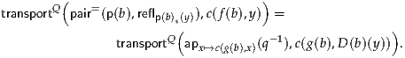 |
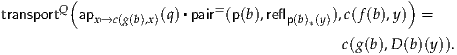
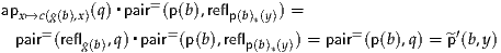 |

Lemma 6.12.4 almost gives ∑(w:W) P(w) the same induction principle as
 . The missing bit is the equality apdf(
 ′(b, y)) = p(b, y). In order to prove
this, we would need to analyze the proof of Lemma 6.12.4, which of course is
the definition of k.
′(b, y)) = p(b, y). In order to prove
this, we would need to analyze the proof of Lemma 6.12.4, which of course is
the definition of k.
It should be possible to do this, but it turns out that we only need the computation rule for the non-dependent recursion principle. Thus, we now give a somewhat simpler direct construction of the recursor, and a proof of its computation rule.
Lemma 6.12.5. Suppose Qis a type and that we have
 c(f(b), y) = Qc(g(b), D(b)(y))
 .
.Then there exists k :  ∑(w:W) P(w)
 → Qsuch that k(
 ′(a, x)) ≡ c(a, x).
Proof. As in Lemma 6.12.4, we define k(w, x) by induction on w : W. When w ≡c(a), we define k(c(a), x) :≡ c(a, x). Now by Lemma 2.9.6, it suffices to consider, for b : B and y : C(f(b)), the composite path
 | (6.12.6) |
defined as the composition
transportx Q(p(b), c(f(b), y)) Q(p(b), c(f(b), y)) | = c(f(b), y) | (by Lemma 2.3.5) |
| = c(g(b), D(b)(y)) | (by p(b, y)) | |
| = c(g(b), transportP(p(b), y)). | (by Lemma 6.12.1) |
 ′(a, x)) ≡ c(a, x) follows by definition, as
before. __
′(a, x)) ≡ c(a, x) follows by definition, as
before. __
For the second computation rule, we need the following lemma.
Lemma 6.12.7. Let Y : X →be a type family and let k : ( ∑(x:X) Y(x)) →
Z be defined componentwise by k(x, y) :≡ d(x)(y) for a curried function
d : ∏(x:X) Y(x) → Z. Then for any s : x1 =X x2 and any y1 : Y(x1) and
y2 : Y(x2) with a path r : s* = y2, the path

is equal to the composite
| k(x1, y1) | ≡ d(x1)(y1) | ||
= transportx Z(s, d(x1)(y1)) Z(s, d(x1)(y1)) | (by (Lemma 2.3.5)-1) | ||
= transportx Z(s, d(x1)(s-1
* Z(s, d(x1)(s-1
* )) )) | |||
=  transportx transportx (Y(x)→Z)(s, d(x1)) (Y(x)→Z)(s, d(x1)) (s
* (s
* ) ) | (by (2.9.4)) | ||
= d(x2)(s* ) ) | (by happly (apd d (s))(s* ) )
| ||
| = d(x2)(y2) | (by apd(x2)(r)) | ||
| ≡ k(x2, y2). |
Proof. After path induction on s and r, both equalities reduce to reflexivities. __
At first it may seem surprising that Lemma 6.12.7 has such a complicated statement, while it can be proven so simply. The reason for the complication is to ensure that the statement is well-typed: apk(pair=(s, r)) and the composite path it is claimed to be equal to must both have the same start and end points. Once we have managed this, the proof is easy by path induction.
Lemma 6.12.8. In the situation of Lemma 6.12.5, we have apk( ′(b, y)) =
p(b, y).
′(b, y)) =
p(b, y).
Proof. Recall that  ′(b, y) :≡pair=(p(b), q) where q : p(b)*
 = D(b)(y)
comes from Lemma 6.12.1. Thus, since k is defined componentwise, we may
compute apk(
= D(b)(y)
comes from Lemma 6.12.1. Thus, since k is defined componentwise, we may
compute apk( ′(b, y)) by Lemma 6.12.7, with
| x1 | :≡c(f(b)) | y1 | :≡ y | ||||
| x2 | :≡c(g(b)) | y2 | :≡ D(b)(y) | ||||
| s | :≡p(b) | r | :≡ q. |
 ).
).
For the first, since d(c(a), x) ≡ c(a, x), we have
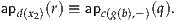
For the second, the computation rule for the induction principle of W tells us
that apdd(p(b)) is equal to the composite (6.12.6), passed across the
equivalence of Lemma 2.9.6. Thus, the computation rule given in
Lemma 2.9.6 implies that happly(apdd(p(b)), p(b)* ) is equal to the
composite
) is equal to the
composite
 p(b)* p(b)*  (p(b)* (p(b)* ) ) | = p(b)* | (by (2.9.4)) | |
= p(b)* | |||
| = c(f(b), y) | (by Lemma 2.3.5) | ||
| = c(f(b), D(b)(y)) | (by p(b, y)) | ||
= c(f(b), p(b)* ). ). | (by ap c(g(b),-) (q) -1) |
 ) into
Lemma 6.12.7, we see that all the paths cancel out in pairs, leaving only
p(b, y). __
) into
Lemma 6.12.7, we see that all the paths cancel out in pairs, leaving only
p(b, y). __
Now we are finally ready to prove the flattening lemma.
Proof of Lemma 6.12.2. We define h :  → ∑(w:W) P(w) by using the
recursion principle for
→ ∑(w:W) P(w) by using the
recursion principle for  , with
  ′ and
′ and  ′ as input data. Similarly, we
define k : ( ∑(w:W) P(w)) →
′ as input data. Similarly, we
define k : ( ∑(w:W) P(w)) →  by using the recursion principle of
Lemma 6.12.5, with
by using the recursion principle of
Lemma 6.12.5, with  and
and  as input data.
On the one hand, we must show that for any z :  , we have
k(h(z)) = z. By induction on z, it suffices to consider the two constructors
of
, we have
k(h(z)) = z. By induction on z, it suffices to consider the two constructors
of  . But we have

by definition, while similarly

using the propositional computation rule for  and Lemma 6.12.8.
On the other hand, we must show that for any z : ∑(w:W) P(w), we have h(k(z)) = z. But this is essentially identical, using Lemma 6.12.4 for “induction on ∑(w:W) P(w)” and the same computation rules. __
In §5.6, we discussed the conditions on a putative “inductive definition” which make it acceptable, namely that all inductive occurrences of the type in its constructors are “strictly positive”. In this section, we say something about the additional conditions required for higher inductive definitions. Finding a general syntactic description of valid higher inductive definitions is an area of current research, and all of the solutions proposed to date are somewhat technical in nature; thus we only give a general description and not a precise definition. Fortunately, the corner cases never seem to arise in practice.
Like an ordinary inductive definition, a higher inductive definition is specified by a list of constructors, each of which is a (dependent) function. For simplicity, we may require the inputs of each constructor to satisfy the same condition as the inputs for constructors of ordinary inductive types. In particular, they may contain the type being defined only strictly positively. Note that this excludes definitions such as the 0-truncation as presented in §6.9, where the input of a constructor contains not only the inductive type being defined, but its identity type as well. It may be possible to extend the syntax to allow such definitions; but also, in §7.3 we will give a different construction of the 0-truncation whose constructors do satisfy the more restrictive condition.
The only difference between an ordinary inductive definition and a higher one, then, is that the output type of a constructor may be, not the type being defined (W, say), but some identity type of it, such as u =W v, or more generally an iterated identity type such as p =(u=Wv) q. Thus, when we give a higher inductive definition, we have to specify not only the inputs of each constructor, but the expressions u and v (or u, v, p, and q, etc.) which determine the source and target of the path being constructed.
Importantly, these expressions may refer to other constructors of W. For instance, in the definition of S1, the constructor loop has both u and v being base, the previous constructor. To make sense of this, we require the constructors of a higher inductive type to be specified in order, and we allow the source and target expressions u and v of each constructor to refer to previous constructors, but not later ones. (Of course, in practice the constructors of any inductive definition are written down in some order, but for ordinary inductive types that order is irrelevant.)
Note that this order is not necessarily the order of “dimension”: in principle, a 1-dimensional path constructor could refer to a 2-dimensional one and hence need to come after it. However, we have not given the 0-dimensional constructors (point constructors) any way to refer to previous constructors, so they might as well all come first. And if we use the hub-and-spoke construction (§6.7) to reduce all constructors to points and 1-paths, then we might assume that all point constructors come first, followed by all 1-path constructors — but the order among the 1-path constructors continues to matter.
The remaining question is, what sort of expressions can u and v be? We might hope that they could be any expression at all involving the previous constructors. However, the following example shows that a naive approach to this idea does not work.
Example 6.13.1. Consider a family of functions f : ∏(X:) (X → X). Of
course, fX might be just idX for all X, but other such fs may also exist.
For instance, nothing prevents f2 : 2 → 2 from being the nonidentity
automorphism (see Exercise 6.9).
Now suppose that we attempt to define a higher inductive type K generated by:
What would the induction principle for K say? We would assume a type family
P : K →, and of course we would need x : P(a) and y : P(b). The remaining
datum should be a dependent path in P living over σ, which must therefore
connect some element of P(fK(a)) to some element of P(fK(b)). But what
could these elements possibly be? We know that P(a) and P(b) are inhabited
by x and y, respectively, but this tells us nothing about P(fK(a)) and
P(fK(b)).
Clearly some condition on u and v is required in order for the definition to be sensible. It seems that, just as the domain of each constructor is required to be (among other things) a covariant functor, the appropriate condition on the expressions u and v is that they define natural transformations. Making precise sense of this requirement is beyond the scope of this book, but informally it means that u and v must only involve operations which are preserved by all functions between types.
For instance, it is permissible for u and v to refer to concatenation of paths, as in the case of the final constructor of the torus in §6.6, since all functions in type theory preserve path concatenation (up to homotopy). However, it is not permissible for them to refer to an operation like the function f in Example 6.13.1, which is not necessarily natural: there might be some function g : X → Y such that fY∘g≠g∘fX. (Univalence implies that fX must be natural with respect to all equivalences, but not necessarily with respect to functions that are not equivalences.)
The intuition of naturality supplies only a rough guide for when a higher inductive definition is permissible. Even if it were possible to give a precise specification of permissible forms of such definitions in this book, such a specification would probably be out of date quickly, as new extensions to the theory are constantly being explored. For instance, the presentation of n-spheres in terms of “dependent n-loops” referred to in §6.4, and the “higher inductive-recursive definitions” used in Chapter 11, were innovations introduced while this book was being written. We encourage the reader to experiment — with caution.
The general idea of higher inductive types was conceived in discussions between Andrej Bauer, Peter Lumsdaine, Mike Shulman, and Michael Warren at the Oberwolfach meeting in 2011, although there are some suggestions of some special cases in earlier work. Subsequently, Guillaume Brunerie and Dan Licata contributed substantially to the general theory, especially by finding convenient ways to represent them in computer proof assistants and do homotopy theory with them (see Chapter 8).
A general discussion of the syntax of higher inductive types, and their semantics in higher-categorical models, appears in [LS13b]. As with ordinary inductive types, models of higher inductive types can be constructed by transfinite iterative processes; a slogan is that ordinary inductive types describe free monads while higher inductive types describe presentations of monads.The introduction of path constructors also involves the model-category-theoretic equivalence between “right homotopies” (defined using path spaces) and “left homotopies” (defined using cylinders) — the fact that this equivalence is generally only up to homotopy provides a semantic reason to prefer propositional computation rules for path constructors.
Another (temporary) reason for this preference comes from the limitations of existing computer implementations. Proof assistants like Coq and Agda have ordinary inductive types built in, but not yet higher inductive types. We can of course introduce them by assuming lots of axioms, but this results in only propositional computation rules. However, there is a trick due to Dan Licata which implements higher inductive types using private data types; this yields judgmental rules for point constructors but not path constructors.
The type-theoretic description of higher spheres using loop spaces and suspensions in §§6.4 and 6.5 is largely due to Brunerie and Licata; Hou has given a type-theoretic version of the alternative description that uses n-dimensional paths. The reduction of higher paths to 1-dimensional paths with hubs and spokes (§6.7) is due to Lumsdaine and Shulman. The description of truncation as a higher inductive type is due to Lumsdaine; the (-1)-truncation is closely related to the “bracket types” of [AB04]. The flattening lemma was first formulated in generality by Brunerie.
Quotient types are unproblematic in extensional type theory, such as NuPRL [CAB+86]. They are often added by passing to an extended system of setoids. However, quotients are a trickier issue in intensional type theory (the starting point for homotopy type theory), because one cannot simply add new propositional equalities without specifying how they are to behave. Some solutions to this problem have been studied [Hof95, Alt99, AMS07], and several different notions of quotient types have been considered. The construction of set-quotients using higher-inductives provides an argument for our particular approach (which is similar to some that have previously been considered), because it arises as an instance of a general mechanism. Our construction does not yet provide a new solution to all the computational problems related to quotients, since we still lack a good computational understanding of higher inductive types in general—but it does mean that ongoing work on the computational interpretation of higher inductives applies to the quotients as well. The construction of quotients in terms of equivalence classes is, of course, a standard set-theoretic idea, and a well-known aspect of elementary topos theory; its use in type theory (which depends on the univalence axiom, at least for mere propositions) was proposed by Voevodsky. The fact that quotient types in intensional type theory imply function extensionality was proved by [Hof95], inspired by the work of [Car95] on exact completions; Lemma 6.3.2 is an adaptation of such arguments.
Exercise 6.1. Define concatenation of dependent paths, prove that application of dependent functions preserves concatenation, and write out the precise induction principle for the torus T2 with its computation rules.
Exercise 6.2. Prove that ΣS1 ≃ S2, using the explicit definition of S2 in terms of base and surf given in §6.4.
Exercise 6.3. Prove that the torus T2 as defined in §6.6 is equivalent to S1 ×S1. (Warning: the path algebra for this is rather difficult.)
Exercise 6.4. Define dependent n-loops and the action of dependent functions on n-loops, and write down the induction principle for the n-spheres as defined at the end of §6.4.
Exercise 6.5. Prove that ΣSn ≃Sn+1, using the definition of Sn in terms of Ωn from §6.4.
Exercise 6.7. Prove that if G is a monoid and x : G, then ∑(y:G) ((x⋅y = e) × (y⋅x = e)) is a mere proposition. Conclude, using the principle of unique choice (Corollary 3.9.2), that it would be equivalent to define a group to be a monoid such that for every x : G, there merely exists a y : G such that x⋅y = e and y⋅x = e.
Exercise 6.8. Prove that if A is a set, then List(A) is a monoid. Then complete the proof of Lemma 6.11.5.
Exercise 6.9. Assuming LEM, construct a family f : ∏(X:) (X → X)
such that f2 : 2 →2 is the nonidentity automorphism.
Exercise 6.10. Show that the map constructed in Lemma 6.3.2 is in fact a quasi-inverse to happly, so that an interval type implies the full function extensionality axiom. (You may have to use Exercise 2.16.)
Exercise 6.12. Show that Z ≃N + 1 + N. Show that if we were to define Z as N + 1 + N, then we could obtain Lemma 6.10.12 with judgmental computation rules.
Exercise 6.13. Show that we can also prove Lemma 6.3.2 by using  instead of I.
One of the basic notions of homotopy theory is that of a homotopy n-type: a space containing no interesting homotopy above dimension n. For instance, a homotopy 0-type is essentially a set, containing no nontrivial paths, while a homotopy 1-type may contain nontrivial paths, but no nontrivial paths between paths. Homotopy n-types are also called n-truncated spaces. We have mentioned this notion already in §3.1; our first goal in this chapter is to give it a precise definition in homotopy type theory.
A dual notion to truncatedness is connectedness: a space is n-connected if it has no interesting homotopy in dimensions n and below. For instance, a space is 0-connected (also called just “connected”) if it has only one connected component, and 1-connected (also called “simply connected”) if it also has no nontrivial loops (though it may have nontrivial higher loops between loops).
The duality between truncatedness and connectedness is most easily seen by extending both notions to maps. We call a map n-truncated or n-connected if all its fibers are so. Then n-connected and n-truncated maps form the two classes of maps in an orthogonal factorization system, i.e. every map factors uniquely as an n-connected map followed by an n-truncated one.
In the case n = -1, the n-truncated maps are the embeddings and the n-connected maps are the surjections, as defined in §4.6. Thus, the n-connected factorization system is a massive generalization of the standard image factorization of a function between sets into a surjection followed by an injection. At the end of this chapter, we sketch briefly an even more general theory: any type-theoretic modality gives rise to an analogous factorization system.
As mentioned in §§3.1 and 3.11, it turns out to be convenient to define n-types starting two levels below zero, with the (-1)-types being the mere propositions and the (-2)-types the contractible ones.
Definition 7.1.1. Define the predicate is-n-type : → for n ≥-2 by
recursion as follows:
We say that X is an n-type, or sometimes that it is n-truncated, if is-n-type(X) is inhabited.
Remark 7.1.2. The number n in Definition 7.1.1 ranges over all integers greater than or equal to -2. We could make sense of this formally by defining a type Z≥-2 of such integers (a type whose induction principle is identical to that of N), or instead defining a predicate is-(k- 2)-type for k : N. Either way, we can prove theorems about n-types by induction on n, with n = -2 as the base case.
Example 7.1.3. We saw in Lemma 3.11.10 that X is a (-1)-type if and only if it is a mere proposition. Therefore, X is a 0-type if and only if it is a set.
We have also seen that there are types which are not sets (Example 3.1.9). So far, however, we have not shown for any n > 0 that there exist types which are not n-types. In Chapter 8, however, we will show that the (n + 1)-sphere Sn+1 is not an n-type. (Kraus has also shown that the nth nested univalent universe is also not an n-type, without using any higher inductive types.) Moreover, in §8.8 will give an example of a type that is not an n-type for any (finite) number n.
We begin the general theory of n-types by showing they are closed under certain operations and constructors.
Theorem 7.1.4. Let p : X → Y be a retraction and suppose that X is an n-type, for any n ≥-2. Then Y is also an n-type.
Proof. We proceed by induction on n. The base case n = -2 is handled by Lemma 3.11.7.
For the inductive step, assume that any retract of an n-type is an n-type, and that X is an (n + 1)-type. Let y, y′ : Y; we must show that y = y′ is an n-type. Let s be a section of p, and let ϵ be a homotopy ϵ : p∘s ~ 1. Since X is an (n + 1)-type, s(y) =X s(y′) is an n-type. We claim that y = y′ is a retract of s(y) =X s(y′). For the section, we take

For the retraction, we define t : (s(y) = s(y′)) → (y = y′) by
To show that t is a retraction of aps, we must show that
for any r : y = y′. But this follows from Lemma 2.4.3. __
As an immediate corollary we obtain the stability of n-types under equivalence (which is also immediate from univalence):
Recall also the notion of embedding from §4.6.
Proof. Let x, x′ : X; we must show that x =X x′ is an (n- 1)-type. But since f is an embedding, we have (x =X x′) ≃ (f(x) =Y f(x′)), and the latter is an (n- 1)-type by assumption. __
Note that this theorem fails when n = -2: the map 0 →1 is an embedding, but 1 is a (-2)-type while 0 is not.
Theorem 7.1.7. The hierarchy of n-types is cumulative in the following sense: given a number n ≥-2, if X is an n-type, then it is also an (n + 1)-type.
Proof. We proceed by induction on n.
For n = -2, we need to show that a contractible type, say, A, has contractible path spaces. Let a0 : A be the center of contraction of A, and let x, y : A. We show that x =A y is contractible. By contractibility of A we have a path contrx ▪contry-1 : x = y, which we choose as the center of contraction for x = y. Given any p : x = y, we need to show p = contrx ▪contry-1. By path induction, it suffices to show that reflx = contrx ▪contrx-1, which is trivial.
For the inductive step, we need to show that x =X y is an (n + 1)-type, provided that X is an (n + 1)-type. Applying the inductive hypothesis to x =X y yields the desired result. __
We now show that n-types are preserved by most of the type forming operations.
Theorem 7.1.8. Let n ≥-2, and let A : and B : A →. If Ais an n-type
and for all a : A, B(a) is an n-type, then so is ∑(x:A) B(x).
Proof. We proceed by induction on n.
For n = -2, we choose the center of contraction for ∑(x:A) B(x) to be the pair (a0, b0), where a0 : A is the center of contraction of A and b0 : B(a0) is the center of contraction of B(a0). Given any other element (a, b) of ∑(x:A) B(x), we provide a path (a, b) = (a0, b0) by contractibility of A and B(a0), respectively.
For the inductive step, suppose that A is an (n + 1)-type and for any a : A, B(a) is an (n + 1)-type. We show that ∑(x:A) B(x) is an (n + 1)-type: fix (a1, b1) and (a2, b2) in ∑(x:A) B(x), we show that (a1, b1) = (a2, b2) is an n-type. By Theorem 2.7.2 we have
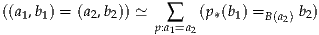
and by preservation of n-types under equivalences (Corollary 7.1.5) it suffices to prove that the latter is an n-type. This follows from the inductive hypothesis. __
As a special case, if A and B are n-types, so is A×B. Note also that Theorem 7.1.7 implies that if A is an n-type, then so is x =A y for any x, y : A. Combining this with Theorem 7.1.8, we see that for any functions f : A → C and g : B → C between n-types, their pullback
(see Exercise 2.11) is also an n-type. More generally, n-types are closed under all limits.
Theorem 7.1.9. Let n ≥-2, and let A : and B : A →. If for all a : A,
B(a) is an n-type, then so is ∏(x:A) B(x).
Proof. We proceed by induction on n. For n = -2, the result is simply Lemma 3.11.6.
For the inductive step, assume the result is true for n-types, and that each B(a) is an (n + 1)-type. Let f, g : ∏(a:A) B(a). We need to show that f = g is an n-type. By function extensionality and closure of n-types under equivalence, it suffices to show that ∏(a:A) (f(a) =B(a) g(a)) is an n-type. This follows from the inductive hypothesis. __
As a special case of the above theorem, the function space A → B is an n-type provided that B is an n-type. We can now generalize our observations in Chapter 2 that isSet(A) and isProp(A) are mere propositions.
Proof. We proceed by induction with respect to n.
For the base case, we need to show that for any X, the type isContr(X) is a mere proposition. This is Lemma 3.11.4.
For the inductive step we need to show

To show the conclusion of this implication, we need to show that for any type X, the type
is a mere proposition. By Example 3.6.2 or Theorem 7.1.9, it suffices to show that for any x, x′ : X, the type is-n-type(x = Xx′) is a mere proposition. But this follows from the inductive hypothesis applied to the type (x = Xx′). __
Finally, we show that the type of n-types is itself an (n + 1)-type. We define this to be:
If necessary, we may specify the universe by writing n-Type . In
particular, we have Prop :≡ (-1)-Type and Set :≡ 0-Type, as defined in
Chapter 2. Note that just as for Prop and Set, because is-n-type(X) is a
mere proposition, by Lemma 3.5.1 for any (X, p), (X′, p′) : n-Type we
have
 (X, p) =n-Type (X′, p′) (X, p) =n-Type (X′, p′) | ≃ (X = X′) | ||
| ≃ (X ≃ X′). |
Proof. Let (X, p), (X′, p′) : n-Type; we need to show that (X, p) = (X′, p′) is an n-type. By the above observation, this type is equivalent to X ≃ X′. Next, we observe that the projection
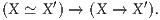
is an embedding, so that if n ≥-1, then by Theorem 7.1.6 it suffices to show that X → X′ is an n-type. But since n-types are preserved under the arrow type, this reduces to an assumption that X′ is an n-type.
In the case n = -2, this argument shows that X ≃ X′ is a (-1)-type — but it is also inhabited, since any two contractible types are equivalent to 1, and hence to each other. Thus, X ≃ X′ is also a (-2)-type. __
In §3.1 we defined a type X to be a set if for all x, y : X and p, q : x = Xy we have p = q. In conventional type theory, this property goes by the name of uniqueness of identity proofs (UIP). We have seen also that it is equivalent to being a 0-type in the sense of the previous section. Here is another equivalent characterization, involving Streicher’s “Axiom K” [Str93]:
Theorem 7.2.1. A type X is a set if and only if it satisfies Axiom K: for all x : X and p : (x = Ax) we have p = reflx.
Proof. Clearly Axiom K is a special case of UIP. Conversely, if X satisfies Axiom K, let x, y : X and p, q : (x = y); we want to show p = q. But induction on q reduces this goal precisely to Axiom K. __
We stress that we are not assuming UIP or the K principle as axioms! They are simply properties which a particular type may or may not satisfy (which are equivalent to being a set). Recall from Example 3.1.9 that not all types are sets.
The following theorem is another useful way to show that types are sets.
Theorem 7.2.2. Suppose R is a reflexive mere relation on a type X implying identity. Then X is a set, and R(x, y) is equivalent to x =X yfor all x, y : X.
Proof. Let ρ : ∏(x:X) R(x, x) witness reflexivity of R, and let
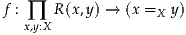 |
be a witness that R implies identity. Note first that the two statements in the theorem are equivalent. For on one hand, if X is a set, then x =X y is a mere proposition, and since it is logically equivalent to the mere proposition R(x, y) by hypothesis, it must also be equivalent to it. On the other hand, if x =X y is equivalent to R(x, y), then like the latter it is a mere proposition for all x, y : X, and hence X is a set.
We give two proofs of this theorem. The first shows directly that X is a set; the second shows directly that R(x, y) ≃ (x = y).
First proof: we show that X is a set. The idea is the same as that of Lemma 3.3.4: the function f must be continuous in its arguments x and y. However, it is slightly more notationally complicated because we have to deal with the additional argument of type R(x, y).
Firstly, for any x : X and p : x =X x, consider apdf(x)(p). This is a dependent path from f(x, x) to itself. Since f(x, x) is still a function R(x, x) → (x =X y), by Lemma 2.9.6 this yields for any r : R(x, x) a path

On the left-hand side, we have transport in an identity type, which is
concatenation. And on the right-hand side, we have p* = r, since both
lie in the mere proposition R(x, x). Thus, substituting r :≡ ρ(x), we
obtain
= r, since both
lie in the mere proposition R(x, x). Thus, substituting r :≡ ρ(x), we
obtain

By cancellation, p = reflx. So X satisfies Axiom K, and hence is a set.
Second proof: we show that each f(x, y) : R(x, y) → x =X y is an equivalence. By Theorem 4.7.7, it suffices to show that f induces an equivalence of total spaces:
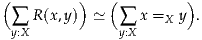 |
By Lemma 3.11.8, the type on the right is contractible, so it suffices to show that the type on the left is contractible. As the center of contraction we take the pair (x, ρ(x)). It remains to show, for every y : X and every H : R(x, y) that
 |
But since R(x, y) is a mere proposition, by Theorem 2.7.2 it suffices to show that x =X y, which we get from f(H). __
Corollary 7.2.3. If a type X has the property that ¬¬(x = y) → (x = y) for any x, y : X, then X is a set.
Another convenient way to show that a type is a set is the following. Recall from §3.4 that a type X is said to have decidable equality if for all x, y : X we have
This is a very strong condition: it says that a path x = y can be chosen, when it exists, continuously (or computably, or functorially) in x and y. This turns out to imply that X is a set, by way of Theorem 7.2.2 and the following lemma.
Proof. Suppose x : A + ¬A. We have two cases to consider. If x is inl(a) for some a : A, then we have the constant function ¬¬A → A which maps everything to a. If x is inr(t) for some t : ¬A, we have g(t) : 0 for every g : ¬¬A. Hence we may use ex falso quodlibet, that is rec0, to obtain an element of A for any g : ¬¬A. __
Proof. If X has decidable equality, it follows that ¬¬(x = y) → (x = y) for any x, y : X. Therefore, Hedberg’s theorem follows from Corollary 7.2.3. __
There is, of course, a strong connection between this theorem and Corollary 3.2.7. The statement LEM∞ that is denied by Corollary 3.2.7 clearly implies that every type has decidable equality, and hence is a set, which we know is not the case. Note that the consistent axiom LEM from §3.4 implies only that every type has merely decidable equality, i.e. that for any A we have
As an example application of Theorem 7.2.5, recall that in Example 3.1.4 we observed that N is a set, using our characterization of its equality types in §2.13. A more traditional proof of this theorem uses only (2.13.2) and (2.13.3), rather than the full characterization of Theorem 2.13.1, with Theorem 7.2.5 to fill in the blanks.
Proof. Let x, y : N be given; we proceed by induction on x and case analysis on y to prove (x = y) + ¬(x = y). If x ≡ 0 and y ≡ 0, we take inl(refl0). If x ≡ 0 and y ≡ succ(n), then by (2.13.2) we get ¬(0 = succ(n)).
For the inductive step, let x ≡succ(n). If y ≡ 0, we use (2.13.2) again.
Finally, if y ≡succ(m), the inductive hypothesis gives (m = n) + ¬(m =
n). In the first case, if p : m = n, then succ : succ(m) = succ(n). And
in the second case, (2.13.3) yields ¬(succ(m) = succ(n)). __
: succ(m) = succ(n). And
in the second case, (2.13.3) yields ¬(succ(m) = succ(n)). __
Although Hedberg’s theorem appears rather special to sets (0-types), “Axiom K” generalizes naturally to n-types. Note that the ordinary Axiom K (as a property of a type X) states that for all x : X, the loop space Ω(X, x) (see Definition 2.1.8) is contractible. Since Ω(X, x) is always inhabited (by reflx), this is equivalent to its being a mere proposition (a (-1)-type). Since 0 = (-1) + 1, this suggests the following generalization.
Theorem 7.2.7. For any n ≥-1, a type X is an (n + 1)-type if and only if for all x : X, the type Ω(X, x) is an n-type.
Before proving this, we prove an auxiliary lemma:
Lemma 7.2.8. Given n ≥ -1 and X : . If, given any inhabitant of X it
follows that X is an n-type, then X is an n-type.
Proof. Let f : X →is-n-type(X) be the given map. We need to show that for any x, x′ : X, the type x = x′ is an (n- 1)-type. But then f(x) shows that X is an n-type, hence all its path spaces are (n- 1)-types. __
Proof of Theorem 7.2.7. The “only if” direction is obvious, since Ω(X, x) :≡ (x =X x). Conversely, in order to show that X is an (n + 1)-type, we need to show that for any x, x′ : X, the type x = x′ is an n-type. Following Lemma 7.2.8 it suffices to give a map
By path induction, it suffices to do this when x ≡ x′, in which case it follows from the assumption that Ω(X, x) is an n-type. __
By induction and some slightly clever whiskering, we can obtain a generalization of the K property to n > 0.
Theorem 7.2.9. For every n ≥ -1, a type A is an n-type if and only if Ωn+1(A, a) is contractible for all a : A.
Proof. Recalling that Ω0(A, a) = (A, a), the case n = -1 is Exercise 3.5. The case n = 0 is Theorem 7.2.1. Now we use induction; suppose the statement holds for n : N. By Theorem 7.2.7, A is an (n + 1)-type iff Ω(A, a) is an n-type for all a : A. By the inductive hypothesis, the latter is equivalent to saying that Ωn+1(Ω(A, a), p) is contractible for all p : Ω(A, a).
Since Ωn+2(A, a) :≡ Ωn+1(Ω(A, a), refla), and Ωn+1 = Ωn∘ Ω, it will
suffice to show that Ω(Ω(A, a), p) is equal to Ω(Ω(A, a), refla), in the
type ∙ of pointed types. For this, it suffices to give an equivalence

which carries the basepoint reflp to the basepoint reflrefla. For q : p = p, define g(q) : refla = refla to be the following composite:
where the path labeled “q” is actually apλr.r▪p-1 (q). Then g is an equivalence because it is a composite of equivalences

using Example 2.4.8 and Theorem 2.11.1, where i : refla = p▪p-1 is the canonical equality. And it is evident that g(reflp) = reflrefla. __
In §3.7 we introduced the propositional truncation, which makes the “best approximation” of a type that is a mere proposition, i.e. a (-1)-type. In §6.9 we constructed this truncation as a higher inductive type, and gave one way to generalize it to a 0-truncation. We now explain a better generalization of this, which truncates any type into an n-type for any n ≥-2; in classical homotopy theory this would be called its nth Postnikov section.
The idea is to make use of Theorem 7.2.9, which states that A is an n-type just when Ωn+1(A, a) is contractible for all a : A, and Lemma 6.5.4, which implies that
 |
where Sn+1 is equipped with some basepoint which we may as well call base. However, contractibility of Map*(Sn+1, (A, a)) is something that we can ensure directly by giving path constructors.
We will use the “hub and spoke” construction as in §6.7. Thus,
for n ≥-1, we take  n to be the higher inductive type generated
by:
n to be the higher inductive type generated
by:
 n,
n,
 n, a hub point h(r) :
  n, and
 n and each x : Sn+1, a spoke path
sr(x) : r(x) = h(r).
n and each x : Sn+1, a spoke path
sr(x) : r(x) = h(r).The existence of these constructors is now enough to show:
Proof. By Theorem 7.2.9, it suffices to show that Ωn+1( n, b) is
contractible for all b :
n, b) is
contractible for all b :  n, which by Lemma 6.5.4 is equivalent
to
n, which by Lemma 6.5.4 is equivalent
to
 |
As center of contraction for the latter, we choose the function cb : Sn+1 → n
which is constant at b, together with reflb : cb(base) = b.
n
which is constant at b, together with reflb : cb(base) = b.
Now, an arbitrary element of Map*(Sn+1, ( n, b)) consists of a map
r : Sn+1 →
n, b)) consists of a map
r : Sn+1 → n together with a path p : r(base) = b. By function
extensionality, to show r = cb it suffices to give, for each x : Sn+1, a path
r(x) = cb(x) ≡ b. We choose this to be the composite sr(x) ▪sr(base)-1 ▪p,
where sr(x) is the spoke at x.
n together with a path p : r(base) = b. By function
extensionality, to show r = cb it suffices to give, for each x : Sn+1, a path
r(x) = cb(x) ≡ b. We choose this to be the composite sr(x) ▪sr(base)-1 ▪p,
where sr(x) is the spoke at x.
Finally, we must show that when transported along this equality r = cb, the path p becomes reflb. By transport in path types, this means we need
But this is immediate from path operations. __
(This construction fails for n = -2, but in that case we can simply define
 -2 :≡1 for all A. From now on we assume n ≥-1.)
To show the desired universal property of the n-truncation, we need the
induction principle. We extract this from the constructors in the usual way; it
says that given P :  n → together with
 n),
n),
 n and r′ : ∏(x:Sn+1) P(r(x)), an element
h′(r, r′) : P(h(r)),
n and r′ : ∏(x:Sn+1) P(r(x)), an element
h′(r, r′) : P(h(r)),
 n and r′ : ∏(x:Sn+1) P(r(x)), and each
x : Sn+1, a dependent path r′(x) =Ps
r(x) h′(r, r′),
n and r′ : ∏(x:Sn+1) P(r(x)), and each
x : Sn+1, a dependent path r′(x) =Ps
r(x) h′(r, r′),there exists a section f : ∏(x:∥A∥n) P(x) with f( n) ≡ g(a) for all a : A. To make
this more useful, we reformulate it as follows.
n) ≡ g(a) for all a : A. To make
this more useful, we reformulate it as follows.
Theorem 7.3.2. For any type family P :  n → such that each P(x)
is an n-type, and any function g : ∏(a:A) P(
n → such that each P(x)
is an n-type, and any function g : ∏(a:A) P( n), there exists a section
f : ∏(x:∥A∥n) P(x) such that f(
n), there exists a section
f : ∏(x:∥A∥n) P(x) such that f( n) :≡ g(a) for all a : A.
Proof. It will suffice to construct the second and third data listed above,
since g has exactly the type of the first datum. Given r : Sn+1 →
 n and r′ : ∏(x:Sn+1) P(r(x)), we have h(r) :
  n and sr :
∏
(x:Sn+1) (r(x) = h(r)). Define t : Sn+1 → P(h(r)) by t(x) :≡
sr(x)
*
n and sr :
∏
(x:Sn+1) (r(x) = h(r)). Define t : Sn+1 → P(h(r)) by t(x) :≡
sr(x)
* . Then since P(h(r)) is n-truncated, there exists a point u :
P(h(r)) and a contraction v : ∏(x:Sn+1) (t(x) = u). Define h′(r, r′) :≡ u,
giving the second datum. Then (recalling the definition of dependent
paths), v has exactly the type required of the third datum. __
. Then since P(h(r)) is n-truncated, there exists a point u :
P(h(r)) and a contraction v : ∏(x:Sn+1) (t(x) = u). Define h′(r, r′) :≡ u,
giving the second datum. Then (recalling the definition of dependent
paths), v has exactly the type required of the third datum. __
In particular, if E is some n-type, we can consider the constant family of
types equal to E for every point of A. Thus, every map f : A → E can be
extended to a map ext(f) :  n → E defined by ext(f)(
 n) :≡ f(a); this is
the recursion principle for
n) :≡ f(a); this is
the recursion principle for  n.
n.
The induction principle also implies a uniqueness principle for functions
of this form. Namely, if E is an n-type and g, g′ :  n → E are such that
g(
n → E are such that
g( n) = g′(
 n) for every a : A, then g(x) = g′(x) for all x :
  n, since
the type g(x) = g′(x) is an n-type. Thus, g = g′. (In fact, this uniqueness
principle holds more generally when E is an (n + 1)-type.) This yields the
following universal property.
n, since
the type g(x) = g′(x) is an n-type. Thus, g = g′. (In fact, this uniqueness
principle holds more generally when E is an (n + 1)-type.) This yields the
following universal property.
Lemma 7.3.3 (Universal property of truncations). Let n ≥-2, A : and
B : n-Type. The following map is an equivalence:
Proof. Given that B is n-truncated, any f : A → B can be extended to a
map ext(f) :  n → B. The map ext(f) ∘|–|n is equal to f, because
for every a : A we have ext(f)(
n → B. The map ext(f) ∘|–|n is equal to f, because
for every a : A we have ext(f)( n) = f(a) by definition. And the map
ext(g∘|–|n) is equal to g, because they both send
n) = f(a) by definition. And the map
ext(g∘|–|n) is equal to g, because they both send  n to g(
 n). __
In categorical language, this says that the n-types form a reflective
subcategory of the category of types. (To state this fully precisely, one ought to
use the language of (∞, 1)-categories.) In particular, this implies that the
n-truncation is functorial: given f : A → B, applying the recursion principle to
the composite A →
→ n yields a map
  n :
n :  n →
n → n. By
definition, we have a homotopy
n. By
definition, we have a homotopy
 | (7.3.4) |
expressing naturality of the maps |–|n.
Uniqueness implies functoriality laws such as  n =
n =  n ∘
n ∘ n
and
n
and  n = id
 n, with attendant coherence laws. We also have higher
functoriality, for instance:
n, with attendant coherence laws. We also have higher
functoriality, for instance:
Lemma 7.3.5. Given f, g : A → B and a homotopy h : f ~ g, there is an induced
homotopy  n :
n :  n ~
n ~ n such that the composite
 | (7.3.6) |
is equal to ap|–|n(h(a)).
Proof. First, we indeed have a homotopy with components ap|–|n(h(a)) :
 n =
n =  n. Composing on either sides with the paths
  n =
n =
 n(
n( n) and
  n =
n =  n(
n( n), which arise from the definitions
of
n), which arise from the definitions
of  n and
n and  n, we obtain a homotopy (
 n ∘|–|n) ~ (
 n ∘
|–|n), and hence an equality by function extensionality. But since (– ∘
|–|n) is an equivalence, there must be a path
n ∘
|–|n), and hence an equality by function extensionality. But since (– ∘
|–|n) is an equivalence, there must be a path  n =
n =  n inducing it,
and the coherence laws for function extensionality imply (7.3.6). __
n inducing it,
and the coherence laws for function extensionality imply (7.3.6). __
The following observation about reflective subcategories is also standard.
Proof. “If” follows from closure of n-types under equivalence. On the
other hand, if A is an n-type, we can define ext(idA) :  n → A.
Then we have ext(idA) ∘|–|n = idA : A → A by definition. In order
to prove that |–|n ∘ext(idA) = id
n → A.
Then we have ext(idA) ∘|–|n = idA : A → A by definition. In order
to prove that |–|n ∘ext(idA) = id n, we only need to prove that
|–|n ∘ext(idA) ∘|–|n = id
n, we only need to prove that
|–|n ∘ext(idA) ∘|–|n = id n ∘|–|n. This is again true:
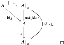
The category of n-types also has some special properties not possessed by
all reflective subcategories. For instance, the reflector  n preserves finite
products.
n preserves finite
products.
Proof. It suffices to show that  n ×
n × n has the same universal property
as
n has the same universal property
as  n. Thus, let C be an n-type; we have
( n × n × n → C) n → C) | = ( n → ( n → ( n → C)) n → C)) | ||
= ( n → (B → C)) n → (B → C)) | |||
| = (A → (B → C)) | |||
| = (A×B → C) |
 n and
n and  n, along with the fact that
B → C is an n-type since C is. It is straightforward to verify that this
equivalence is given by composing with |–|n ×|–|n, as needed. __
n, along with the fact that
B → C is an n-type since C is. It is straightforward to verify that this
equivalence is given by composing with |–|n ×|–|n, as needed. __
The following related fact about dependent sums is often useful.
Proof. We use the induction principle of n-truncation several times to construct functions
| φ | :  ∑
x:A ∑
x:A n n n →
n → ∑
x:AP(x) ∑
x:AP(x) n
n | ||
| ψ | :  ∑
x:AP(x) ∑
x:AP(x) n →
n → ∑
x:A ∑
x:A n n n
n |
 n) :≡
n) :≡ n.
We define ψ by setting ψ(
n.
We define ψ by setting ψ( n) :≡
n) :≡ n. Then we define
H(
n. Then we define
H( n) :≡refl
 n and K(
 n) :≡refl
 n. __
n. __
Proof. If A is an n-type, then the left-hand type above is already an n-type, hence equivalent to its n-truncation; thus this follows from Theorem 7.3.9. __
We can characterize the path spaces of a truncation using the same method that we used in §§2.12 and 2.13 for coproducts and natural numbers (and which we will use in Chapter 8 to calculate homotopy groups). Unsurprisingly, the path spaces in the (n + 1)-truncation of A are the n-truncations of the path spaces of A. Indeed, for any x, y : A there is a canonical map
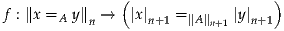 | (7.3.11) |
defined by
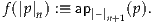
This definition uses the recursion principle for ∥–∥n, which is correct
because  n+1 is (n + 1)-truncated, so that the codomain of f is
n-truncated.
n+1 is (n + 1)-truncated, so that the codomain of f is
n-truncated.
Proof. The proof is a simple application of the encode-decode method:
As in previous situations, we cannot directly define a quasi-inverse to the
map (7.3.11) because there is no way to induct on an equality between
 n+1 and
  n+1. Thus, instead we generalize its type, in order to
have general elements of the type
n+1. Thus, instead we generalize its type, in order to
have general elements of the type  n+1 instead of
  n+1 and
  n+1.
Define P :
n+1.
Define P :  n+1 →
n+1 → n+1 → n-Type by

This definition is correct because  n is n-truncated, and n-Type
is (n + 1)-truncated by Theorem 7.1.11. Now for every u, v :
n is n-truncated, and n-Type
is (n + 1)-truncated by Theorem 7.1.11. Now for every u, v :  n+1,
there is a map
n+1,
there is a map
defined for u =  n+1 and v =
  n+1 and p : x = y by
Since the codomain of decode is n-truncated, it suffices to define it only for u and v of this form, and then it’s just the same definition as before. We also define a function
by induction on u, where r( n+1) :≡
 n.
n.
Now we can define an inverse map
by

To show that the composite

is the identity function, by path induction it suffices to check it for reflu :
u = u, in which case what we need to know is that encode(r(u)) = reflu.
But since this is an n-type, hence also an (n + 1)-type, we may assume
u ≡ n+1, in which case it follows by definition of r and encode. Finally,
to show that
n+1, in which case it follows by definition of r and encode. Finally,
to show that
is the identity function, since this goal is again an n-type, we may
assume that u =  n+1 and v =
  n+1 and that we are considering
 n : P(
 n+1,
n+1,  n+1) for some p : x = y. Then we have
encode(decode( n)) n)) | = encode(ap|–| n+1 (p)) | ||
= transportv P( P( n+1,v)(ap
|–|n+1 (p), n+1,v)(ap
|–|n+1 (p),  n) n) | |||
= transportv  n(p, n(p,  n)
n) | |||
=  n n | |||
=  n. n. |
 n+1 and v =
  n+1. __
Proof. This is a special case of the previous lemma where x = y = a. __
Proof. By induction on k, using the recursive definition of Ωk. __
We also observe that “truncations are cumulative”: if we truncate to an n-type and then to a k-type with k ≤ n, then we might as well have truncated directly to a k-type.
Proof. We define two maps f :  k →
k →  k and g :
  k →
k →
 k by
k by

The map f is well-defined because  k is k-truncated and also
n-truncated (because k ≤ n), and the map g is well-defined because
k is k-truncated and also
n-truncated (because k ≤ n), and the map g is well-defined because
 k is k-truncated.
The composition f ∘g :  k →
k → k satisfies (f ∘g)(
 k) =
k) =  k,
hence f ∘g = id
k,
hence f ∘g = id k. Similarly, we have (g∘f)(
 k) =
k) =  k and
hence g∘f = id
k and
hence g∘f = id k. __
k. __
Recall that in §6.8, we used higher inductive types to define pushouts of types, and proved their universal property. In general, a (homotopy) colimit of n-types may no longer be an n-type (for an extreme counterexample, see Exercise 7.2). However, if we n-truncate it, we obtain an n-type which satisfies the correct universal property with respect to other n-types.
In this section we prove this for pushouts, which are the most important and nontrivial case of colimits. Recall the following definitions from §6.8.
Definition 7.4.2. Given a span = (A, B, C, f, g) and a type D, a cocone
under with base D is a triple (i, j, h) with i : A → D, j : B → D and
h : ∏(c:C) i(f(c)) = j(g(c)):

We denote by cocone (D) the type of all such cocones.
The type of cocones is (covariantly) functorial. For instance, given D, E and a map t : D → E, there is a map
defined by:

And given D, E, F, functions t : D → E, u : E → F and c : cocone (D), we
have
| idD ∘c | = c | (7.4.3) |
| (u∘t) ∘c | = u∘ (t∘c). | (7.4.4) |
Definition 7.4.5. Given a span of n-types, an n-type D, and a cocone
c : cocone (D), the pair (D, c) is said to be a pushout of in n-types if
for every n-type E, the map
is an equivalence.
In order to construct pushouts of n-types, we need to explain how to reflect spans and cocones.
Definition 7.4.7. Let D : and c = (i, j, h) : cocone (D). We define

where  n :
n :  n ∘
n ∘ n ~
n ~  n ∘
n ∘ n is defined as in
Lemma 7.3.5.
n is defined as in
Lemma 7.3.5.
We now observe that the maps from each type to its n-truncation assemble into a map of spans, in the following sense.
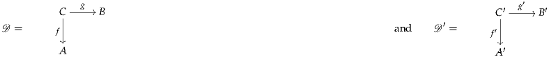
be spans. A map of spans → ′ consists of functions α : A → A′,
β : B → B′, and γ : C → C′ and homotopies ϕ : α∘f ~ f′∘γ and
ψ : β∘g ~ g′∘γ.
Thus, for any span , we have a map of spans |–|n : → n
consisting of |–|An, |–|Bn, |–|Cn, and the naturality homotopies natnf and natng
from (7.3.4).
n
consisting of |–|An, |–|Bn, |–|Cn, and the naturality homotopies natnf and natng
from (7.3.4).
We also need to know that maps of spans behave functorially. Namely, if
(α, β, γ, ϕ, ψ) : → ′ is a map of spans and D any type, then we
have
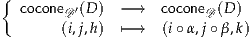
where k : ∏(z:C) i(α(f(z))) = j(β(g(z))) is the composite
 | (7.4.9) |
We denote this cocone by (i, j, h) ∘ (α, β, γ, ϕ, ψ). Moreover, this functorial action commutes with the other functoriality of cocones:
Proof. Given (i, j, h) : cocone ′(D), note that both composites yield a cocone
whose first two components are t∘i∘α and t∘j∘β. Thus, it remains to verify
that the homotopies agree. For the top-right composite, the homotopy
is (7.4.9) with (i, j, h) replaced by (t∘i, t∘j, apt ∘h):
 |
(For brevity, we are omitting the parentheses around the arguments of functions.) On the other hand, for the left-bottom composite, the homotopy is apt applied to (7.4.9). Since ap respects path-concatenation, this is equal to
 |
But apt ∘api = apt∘i and similarly for j, so these two homotopies are equal. __
Finally, note that since we defined  n : cocone
 n(
n( n) using
Lemma 7.3.5, the additional condition (7.3.6) implies
n) using
Lemma 7.3.5, the additional condition (7.3.6) implies
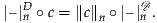 | (7.4.11) |
for any c : cocone (D). Now we can prove our desired theorem.
Proof. Let E be an n-type, and consider the following diagram:
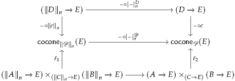 |
The upper horizontal arrow is an equivalence since E is an n-type, while – ∘c
is an equivalence since c is a pushout cocone. Thus, by the 2-out-of-3 property,
to show that – ∘ n is an equivalence, it will suffice to show that the
upper square commutes and that the middle horizontal arrow is an
equivalence. To see that the upper square commutes, let t :
n is an equivalence, it will suffice to show that the
upper square commutes and that the middle horizontal arrow is an
equivalence. To see that the upper square commutes, let t :  n → E;
then
n → E;
then
 t∘ t∘ n n ∘|–|
n ∘|–|
n | = t∘  n ∘|–|
n n ∘|–|
n  | (by Lemma 7.4.10) |
= t∘ |–|Dn ∘c |–|Dn ∘c | (by (7.4.11)) | |
=  t∘|–|Dn t∘|–|Dn ∘c. ∘c. | (by (7.4.4)) |
| ℓ1(i, j, p) | :≡ (i, j, happly(p)) | ||
| ℓ2(i, j, p) | :≡ (i, j, happly(p)) |
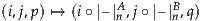 " class="math-display" >
where q is the composite
| i∘|–|An ∘f | = i∘ n ∘|–|Cn n ∘|–|Cn | (by funext(λz.api(natnf(z)))) |
= j∘ n ∘|–|Cn n ∘|–|Cn | (by ap–∘|–|C n (p)) | |
| = j∘|–|Bn ∘g. | (by funext(λz.apj(natng(z)))) |

(with q as above) is equal to the composite
i( n) n) | = i( n( n( n)) n)) | (by api(natnf(z))) |
= j( n( n( n)) n)) | (by happly(p,  n)) n))
| |
= j( n). n). | (by apj(natng(z))) |
| happly(funext(λz.api(natnf(z))), z) | = api(natnf(z)) | ||
| happly(ap–∘|–|C n (p), z) | = happly(p,  n) n) | ||
| happly(funext(λz.apj(natng(z))), z) | = apj(natng(z)). |
An n-type is one that has no interesting information above dimension n. By contrast, an n-connected type is one that has no interesting information below dimension n. It turns out to be natural to study a more general notion for functions as well.
Definition 7.5.1. A function f : A → B is said to be n-connected if for all b : B,
the type  n is contractible:
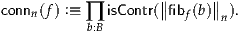 |
A type A is said to be n-connected if the unique function A →1 is
n-connected, i.e. if  n is contractible.
Thus, a function f : A → B is n-connected if and only if fibf(b) is n-connected for every b : B. Of course, every function is (-2)-connected. At the next level, we have:
Lemma 7.5.2. A function f is (-1)-connected if and only if it is surjective in the sense of §4.6.
Proof. We defined f to be surjective if  -1 is inhabited for
all b. But since it is a mere proposition, inhabitation is equivalent to
contractibility. __
-1 is inhabited for
all b. But since it is a mere proposition, inhabitation is equivalent to
contractibility. __
Thus, n-connectedness of a function for n ≥ 0 can be thought of as a strong form of surjectivity. Category-theoretically, (-1)-connectedness corresponds to essential surjectivity on objects, while n-connectedness corresponds to essential surjectivity on k-morphisms for k ≤ n + 1.
Lemma 7.5.2 also implies that a type A is (-1)-connected if and only if it is merely inhabited. When a type is 0-connected we may simply say that it is connected, and when it is 1-connected we say it is simply connected.
Remark 7.5.3. While our notion of n-connectedness for types agrees with the standard notion in homotopy theory, our notion of n-connectedness for functions is off by one from a common indexing in classical homotopy theory. Whereas we say a function f is n-connected if all its fibers are n-connected, some classical homotopy theorists would call such a function (n + 1)-connected. (This is due to a historical focus on cofibers rather than fibers.)
We now observe a few closure properties of connected maps.
Proof. This is a direct consequence of Lemma 4.7.3. __
Lemma 7.5.6. Suppose that f : A → B is n-connected. Then g : B → C is n-connected if and only if g∘f is n-connected.
Proof. For any c : C, we have
 n n | ≃ ∑
w:fibg(c) fibf(pr1w) ∑
w:fibg(c) fibf(pr1w) n
n | (by Exercise 4.4) |
≃ ∑
w:fibg(c) ∑
w:fibg(c)  n n n
n | (by Theorem 7.3.9) | |
≃ n. n. | (since  n is contractible) n is contractible) |
 n is contractible if and only if
  n is
contractible. __
n is
contractible. __
Importantly, n-connected functions can be equivalently characterized as those which satisfy an “induction principle” with respect to n-types. This idea will lead directly into our proof of the Freudenthal suspension theorem in §8.6.
Lemma 7.5.7. For f : A → B and P : B →, consider the following
function:
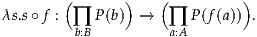 |
For a fixed f and n ≥-2, the following are equivalent.
Proof. Suppose that f is n-connected and let P : B → n-Type. Then we have the equivalences
λs.s∘f. Thus, (i)⇒(ii), and clearly (ii)⇒(iii). To show (iii)⇒(i), consider the type family
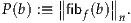 |
Then (iii) yields a map c : ∏(b:B)  n with c(f(a)) =
  n. To
show that each
n. To
show that each  n is contractible, we will find a function of
type
n is contractible, we will find a function of
type
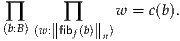 |
By Theorem 7.3.2, for this it suffices to find a function of type
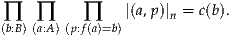 |
But by rearranging variables and path induction, this is equivalent to the type
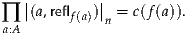 |
This property holds by our choice of c(f(a)). __
Proof. By Theorem 7.3.2 and the associated uniqueness principle, the condition of Lemma 7.5.7 holds. __
For instance, when n = -1, Corollary 7.5.8 says that the map A → from a type to its propositional truncation is surjective.
Corollary 7.5.9. A type Ais n-connected if and only if the map
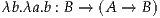 |
is an equivalence for every n-type B. In other words, “every map from Ato an n-type is constant”.
Proof. By Lemma 7.5.7 applied to a function with codomain 1. __
Lemma 7.5.10. Let B be an n-type and let f : A → B be a function. Then
the induced function g :  n → B is an equivalence if and only if f is
n-connected.
n → B is an equivalence if and only if f is
n-connected.
Proof. By Corollary 7.5.8, |–|n is n-connected. Thus, since f = g∘|–|n, by Lemma 7.5.6 f is n-connected if and only if g is n-connected. But since g is a function between n-types, its fibers are also n-types. Thus, g is n-connected if and only if it is an equivalence. __
We can also characterize connected pointed types in terms of connectivity of the inclusion of their basepoint.
Lemma 7.5.11. Let A be a type and a0 : 1 → A a basepoint, with n ≥-1. Then Ais n-connected if and only if the map a0 is (n- 1)-connected.
Proof. First suppose a0 : 1 → A is (n- 1)-connected and let B be an
n-type; we will use Corollary 7.5.9. The map λb.λa.b : B → (A → B) has
a retraction given by f f(a0), so it suffices to show it also has a section,
i.e. that for any f : A → B there is b : B such that f = λa.b. We choose
b :≡ f(a0). Define P : A → by P(a) :≡ (f(a) = f(a0)). Then P is a
family of (n- 1)-types and we have P(a0); hence we have ∏(a:A) P(a)
since a0 : 1 → A is (n- 1)-connected. Thus, f = λa.f(a0) as desired.
f(a0), so it suffices to show it also has a section,
i.e. that for any f : A → B there is b : B such that f = λa.b. We choose
b :≡ f(a0). Define P : A → by P(a) :≡ (f(a) = f(a0)). Then P is a
family of (n- 1)-types and we have P(a0); hence we have ∏(a:A) P(a)
since a0 : 1 → A is (n- 1)-connected. Thus, f = λa.f(a0) as desired.
Now suppose A is n-connected, and let P : A → (n- 1)-Type and u : P(a0) be given. By Lemma 7.5.7, it will suffice to construct f : ∏(a:A) P(a) such that f(a0) = u. Now (n- 1)-Type is an n-type and A is n-connected, so by Corollary 7.5.9, there is an n-type B such that P = λa.B. Hence, we have a family of equivalences g : ∏(a:A) (P(a) ≃ B). Define f(a) :≡ ga-1(ga0(u)); then f : ∏(a:A) P(a) and f(a0) = u as desired. __
In particular, a pointed type (A, a0) is 0-connected if and only if a0 : 1 → A
is surjective, which is to say ∏(x:A)  .
.
A useful variation on Lemma 7.5.6 is:
Lemma 7.5.12. Let f : A → B be a function and P : A →and Q : B →be
type families. Suppose that g : ∏(a:A) P(a) → Q(f(a)) is a fiberwise n-connected
family of functions, i.e. each function ga : P(a) → Q(f(a)) is n-connected. Then the
function
| φ | :  ∑
a:AP(a) ∑
a:AP(a) → → ∑
b:B Q(b) ∑
b:B Q(b) | ||
| φ(a, u) | :≡ (f(a), ga(u)) |
Proof. For b : B and v : Q(b) we have
 n n | ≃ ∑
(a:A) ∑
(u:P(a)) ∑
(p:f(a)=b) f ∑
(a:A) ∑
(u:P(a)) ∑
(p:f(a)=b) f * * = v = v n
n | ||
≃ ∑
(w:fibf(b)) ∑
(u:P(pr1(w))) gpr1w(u) = f ∑
(w:fibf(b)) ∑
(u:P(pr1(w))) gpr1w(u) = f -1
* -1
*  n
n | |||
≃ ∑
w:fibf(b) fibg(pr1w)(f ∑
w:fibf(b) fibg(pr1w)(f -1
* -1
* ) ) n
n | |||
≃ ∑
w:fibf(b) ∑
w:fibf(b) 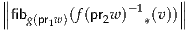 n n n
n | |||
≃ n n |
In the other direction, we have
Lemma 7.5.13. Let P, Q : A →be type families and consider a fiberwise
transformation
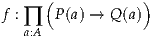 |
from P to Q. Then the induced map total(f) : ∑(a:A) P(a) → ∑(a:A) Q(a) is n-connected if and only if each f(a) is n-connected.
Proof. By Theorem 4.7.6, we have fibtotal(f)((x, v)) ≃fibf(x)(v) for each
x : A and v : Q(x). Hence  n is contractible if and only
if
n is contractible if and only
if  n is contractible. __
Another useful fact about connected maps is that they induce an equivalence on n-truncations:
Proof. Let c be the proof that f is n-connected. From left to right, we
use the map  n :
n :  n →
n →  n. To define the map from right to
left, by the universal property of truncations, it suffices to give a map
back : B →
n. To define the map from right to
left, by the universal property of truncations, it suffices to give a map
back : B → n. We can define this map as follows:
By definition, c(y) has type isContr( n), so its first component
has type
n), so its first component
has type  n, and we can obtain an element of
  n from this
by projection.
n from this
by projection.
Next, we show that the composites are the identity. In both directions, because the goal is a path in an n-truncated type, it suffices to cover the case of the constructor |–|n.
In one direction, we must show that for all x : A,
But  n :
n :  n, and c(f(x)) says that this type is
contractible, so
n, and c(f(x)) says that this type is
contractible, so
Applying  n to both sides of this equation gives the result.
In the other direction, we must show that for all y : B,

pr1(c(y)) has type  n, and the path we want is essentially
the second component of the fibf(y), but we need to make sure the
truncations work out.
n, and the path we want is essentially
the second component of the fibf(y), but we need to make sure the
truncations work out.
In general, suppose we are given p :  n and wish to
prove P(
n and wish to
prove P( n(p)). By truncation induction, it suffices to prove P(
 n)
for all a : A and b : B(a). Applying this principle in this case, it suffices
to prove
n)
for all a : A and b : B(a). Applying this principle in this case, it suffices
to prove
given a : A and b : f(a) = y. But the left-hand side equals  n, so
applying |–|n to both sides of b gives the result. __
n, so
applying |–|n to both sides of b gives the result. __
One might guess that this fact characterizes the n-connected maps, but in fact being n-connected is a bit stronger than this. For instance, the inclusion 02 : 1 →2 induces an equivalence on (-1)-truncations, but is not surjective (i.e. (-1)-connected). In §8.4 we will see that the difference in general is an analogous extra bit of surjectivity.
In set theory, the surjections and the injections form a unique factorization system: every function factors essentially uniquely as a surjection followed by an injection. We have seen that surjections generalize naturally to n-connected maps, so it is natural to inquire whether these also participate in a factorization system. Here is the corresponding generalization of injections.
Definition 7.6.1. A function f : A → B is n-truncated if the fiber fibf(b) is an n-type for all b : B.
In particular, f is (-2)-truncated if and only if it is an equivalence. And of course, A is an n-type if and only if A →1 is n-truncated. Moreover, n-truncated maps could equivalently be defined recursively, like n-types.
Lemma 7.6.2. For any n ≥-2, a function f : A → B is (n + 1)-truncated if and only if for all x, y : A, the map apf : (x = y) → (f(x) = f(y)) is n-truncated. In particular, f is (-1)-truncated if and only if it is an embedding in the sense of §4.6.
Proof. Note that for any (x, p), (y, q) : fibf(b), we have
 (x, p) = (y, q) (x, p) = (y, q) | = ∑ r:x=y (p = apf(r) ▪q) | ||
| = ∑ r:x=y (apf(r) = p▪q-1) | |||
| = fibapf (p▪q-1). |
We can now construct the factorization, in a fairly obvious way.
Definition 7.6.3. Let f : A → B be a function. The n-image of f is defined as
 |
When n = -1, we write simply im(f) and call it the image of f.
Lemma 7.6.4. For any function f : A → B, the canonical function  : A →
imn(f) is n-connected. Consequently, any function factors as an n-connected
function followed by an n-truncated function.
: A →
imn(f) is n-connected. Consequently, any function factors as an n-connected
function followed by an n-truncated function.
Proof. Note that A ≃ ∑(b:B) fibf(b). The function  is the function on total
spaces induced by the canonical fiberwise transformation
is the function on total
spaces induced by the canonical fiberwise transformation
 |
Since each map fibf(b) → n is n-connected by Corollary 7.5.8,
  is
n-connected by Lemma 7.5.13. Finally, the projection pr1 : imn(f) → B is
n-truncated, since its fibers are equivalent to the n-truncations of the fibers of
f. __
is
n-connected by Lemma 7.5.13. Finally, the projection pr1 : imn(f) → B is
n-truncated, since its fibers are equivalent to the n-truncations of the fibers of
f. __
In the following lemma we set up some machinery to prove the unique factorization theorem.
Lemma 7.6.5. Suppose we have a commutative diagram of functions
 |
with H : h1 ∘g1 ~ h2 ∘g2, where g1 and g2 are n-connected and where h1 and h2 are n-truncated. Then there is an equivalence
 |
for any b : B, such that for any a : Awe have an identification

Proof. Let b : B. Then we have the following equivalences:
| fibh1(b) | ≃ ∑
w:fibh1 (b)  n n | (since g1 is n-connected) |
≃ ∑
w:fibh1 (b) fibg1(pr1w) ∑
w:fibh1 (b) fibg1(pr1w) n
n | (by Corollary 7.3.10, since h1 is n-truncated) | |
≃ n n | (by Exercise 4.4) |
 |
for any b : B. By analyzing the underlying functions, we get the following representation of what happens to the element (g1(a), reflh1(g1(a))) after applying each of the equivalences of which E is composed. Some of the identifications are definitional, but others (marked with a = below) are only propositional; putting them together we obtain E(H, a).
| (g1(a), reflh1(g1(a))) |   | ||
  n n | |||
  n n | |||
  n n | |||
  n n | |||
  | |||
 (g2(a), H(a)-1) (g2(a), H(a)-1) |
 |
inserts the center of contraction for  n supplied by the
assumption that g1 is n-truncated; whereas in the case in question this type
has the obvious inhabitant
n supplied by the
assumption that g1 is n-truncated; whereas in the case in question this type
has the obvious inhabitant  n, which by contractibility must be
equal to the center. The second propositional equality is because the
equivalence fibh1∘g1(b) ≃fibh2∘g2(b) concatenates the second components with
H(a)-1, and we have H(a)-1 ▪refl = H(a)-1. The reader may check that the
other equalities are definitional (assuming a reasonable solution to
Exercise 4.4). __
n, which by contractibility must be
equal to the center. The second propositional equality is because the
equivalence fibh1∘g1(b) ≃fibh2∘g2(b) concatenates the second components with
H(a)-1, and we have H(a)-1 ▪refl = H(a)-1. The reader may check that the
other equalities are definitional (assuming a reasonable solution to
Exercise 4.4). __
Combining Lemmas 7.6.4 and 7.6.5, we have the following unique factorization result:
Theorem 7.6.6. For each f : A → B, the space factn(f) defined by
 |
is contractible. Its center of contraction is the element
 |
arising from Lemma 7.6.4, where θ : pr1 ∘ ~ f is the canonical homotopy, where φ
is the proof of Lemma 7.6.4, and where ψ is the obvious proof that pr1 : imn(f) → B
has n-truncated fibers.
~ f is the canonical homotopy, where φ
is the proof of Lemma 7.6.4, and where ψ is the obvious proof that pr1 : imn(f) → B
has n-truncated fibers.
Proof. By Lemma 7.6.4 we know that there is an element of factn(f), hence it is enough to show that factn(f) is a mere proposition. Suppose we have two n-factorizations
 |
of f. Then we have the pointwise-concatenated homotopy

By univalence and the characterization of paths and transport in Σ-types, function types, and path types, it suffices to show that
We prove these four assertions in that order.
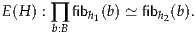 |
This induces an equivalence of total spaces, i.e. we have
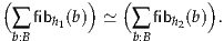 |
Of course, we also have the equivalences X1 ≃ ∑(b:B) fibh1(b) and X2 ≃ ∑(b:B) fibh2(b) from Lemma 4.8.2. This gives us our equivalence e : X1 ≃ X2; the reader may verify that the underlying function of e is given by
 |
 |
giving us a homotopy η : h2 ∘e ~ h1.
By standard arguments, this yields the following orthogonality principle.
Theorem 7.6.7. Let e : A → B be n-connected and m : C → D be n-truncated. Then the map
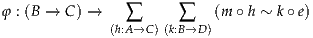
is an equivalence.
Sketch of proof. For any (h, k, H) in the codomain, let h = h2 ∘h1 and k = k2 ∘k1, where h1 and k1 are n-connected and h2 and k2 are n-truncated. Then f = (m∘h2) ∘h1 and f = k2 ∘ (k1 ∘e) are both n-factorizations of m∘h = k∘e. Thus, there is a unique equivalence between them. It is straightforward (if a bit tedious) to extract from this that fibφ((h, k, H)) is contractible. __
We end by showing that images are stable under pullback.
Proof. This follows from pasting of pullbacks (Exercise 2.12), since the type X in the diagram
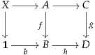 |
is the pullback of the left square if and only if it is the pullback of the outer rectangle, while fibf(b) is the pullback of the square on the left and fibg(h(b)) is the pullback of the outer rectangle. __
Theorem 7.6.9. Consider functions f : A → B, g : C → D and the diagram
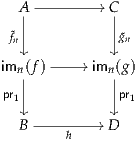 |
If the outer rectangle is a pullback, then so is the bottom square (and hence so is the top square, by Exercise 2.12). Consequently, images are stable under pullbacks.
Proof. Assuming the outer square is a pullback, we have equivalences
| B×Dimn(g) | ≡ ∑ (b:B) ∑ (w:imn(g)) h(b) = pr1w | ||||||
| ≃ ∑ (b:B) ∑ (d:D) ∑ (w:∥fibg(d)∥n) h(b) = d | |||||||
≃ ∑
b:B  n n | |||||||
≃ ∑
b:B  n n | (by Lemma 7.6.8) | ||||||
| ≡imn(f). | __ |
Nearly all of the theory of n-types and connectedness can be done in much greater generality. This section will not be used in the rest of the book.
Our first thought regarding generalizing the theory of n-types might be to take Lemma 7.3.3 as a definition.
Definition 7.7.1. A reflective subuniverse is a predicate P : →Prop
such that for every A : we have a type ◯A such that P(◯A) and a map
ηA : A → ◯A, with the property that for every B : with P(B), the
following map is an equivalence:
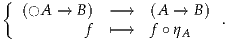
We write P :≡ P(A)}, so A : P means that A : and we
have P(A). We also write rec◯ for the quasi-inverse of the above map.
The notation ◯ may seem slightly odd, but it will make more sense
soon.
P(A)}, so A : P means that A : and we
have P(A). We also write rec◯ for the quasi-inverse of the above map.
The notation ◯ may seem slightly odd, but it will make more sense
soon.
For any reflective subuniverse, we can prove all the familiar facts about reflective subcategories from category theory, in the usual way. For instance, we have:
P if and only if ηA : A →◯A is an equivalence.
P is closed under retracts. In particular, A lies in P as soon as ηA
admits a retraction.
P are closed under all limits such as products and
pullbacks. In particular, for any A : P and x, y : A, the identity
type (x = Ay) is also in P , since it is a pullback of two functions
1 → A.
P can be constructed by applying ◯ to ordinary
colimits of types.Importantly, closure under products extends also to “infinite products”, i.e. dependent function types.
Theorem 7.7.2. If B : A → P is any family of types in a reflective
subuniverse P, then ∏(x:A) B(x) is also in P.
Proof. For any x : A, consider the function evx : ( ∏(x:A) B(x)) → B(x) defined by evx(f) :≡ f(x). Since B(x) lies in P, this extends to a function
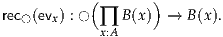
Thus we can define h : ◯( ∏(x:A) B(x)) → ∏(x:A) B(x) by h(z)(x) :≡
rec◯(evx)(z). Then h is a retraction of η∏(x:A) B(x), so that ∏(x:A) B(x) is
in P . __
In particular, if B : P and A is any type, then (A → B) is in P . In
categorical language, this means that any reflective subuniverse is an
exponential ideal. This, in turn, implies by a standard argument that the
reflector preserves finite products.
Corollary 7.7.3. For any types A and B and any reflective subuniverse, the induced map ◯(A×B) →◯(A) ×◯(B) is an equivalence.
Proof. It suffices to show that ◯(A) ×◯(B) has the same universal property as
◯(A×B). Thus, let C : P ; we have
| (◯(A) ×◯(B) → C) | = (◯(A) → (◯(B) → C)) | ||
| = (◯(A) → (B → C)) | |||
| = (A → (B → C)) | |||
| = (A×B → C) |
P since C is. It is straightforward to verify that this equivalence is
given by composing with ηA ×ηB, as needed. __
It may seem odd that every reflective subcategory of types is automatically an exponential ideal, with a product-preserving reflector. However, this is also the case classically in the category of sets, for the same reasons. It’s just that this fact is not usually remarked on, since the classical category of sets—in contrast to the category of homotopy types—does not have many interesting reflective subcategories.
Two basic properties of n-types are not shared by general reflective subuniverses: Theorem 7.1.8 (closure under Σ-types) and Theorem 7.3.2 (truncation induction). However, the analogues of these two properties are equivalent to each other.
Proof. Suppose (i). Then in the situation of (ii), the type ∑(z:◯A) B(z)
lies in P , and we have g′ : A → ∑(z:◯A) B(z) defined by g′(a) :≡
(η(a), g(a)). Thus, we have rec◯(g′) : ◯A → ∑(z:◯A) B(z) such that
rec◯(g′)(η(a)) = (η(a), g(a)).
Now consider the functions pr2 ∘rec◯(g′) : ◯A →◯A and id◯A. By assumption, these become equal when precomposed with η. Thus, by the universal property of ◯, they are equal already, i.e. we have pz : pr2(rec◯(g′)(z)) = z for all z. Now we can define
 |
and the second component of
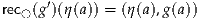 |
yields f(η(a)) = g(a).
Conversely, suppose (ii), and that A : P and B : A →P . Let h be the
composite
Then for z : ∑(x:A) B(x) we have
| h(η(z)) | = η-1(◯(pr 1)(η(z))) | ||
| = η-1(η(pr 1(z))) | |||
| = pr1(z). |
by
C(w) :≡ B(h(w)), we have
Thus, the assumption yields
 |
such that f(η(z)) = g(z). Together, h and f give a function
 |
defined by k(w) :≡ (h(w), f(w)), while pz and the equality f(η(z)) = g(z)
show that k is a retraction of η∑(x:A) B(x). Therefore, ∑(x:A) B(x) is in
P . __
Note the similarity to the discussion in §5.5. The universal property of the
reflector of a reflective subuniverse is like a recursion principle with its
uniqueness property, while Theorem 7.7.4(ii) is like the corresponding
induction principle. Unlike in §5.5, the two are not equivalent here, because of
the restriction that we can only eliminate into types that lie in P .
Condition (i) of Theorem 7.7.4 is what fixes the disconnect.
Unsurprisingly, of course, if we have the induction principle, then we can
derive the recursion principle. We can also derive its uniqueness property, as
long as we allow ourselves to eliminate into path types. This suggests the
following definition. Note that any reflective subuniverse can be characterized
by the operation ◯ : → and the functions ηA : A →◯A, since we have
P(A) = isequiv(ηA).
Definition 7.7.5. A modality is an operation ◯ : → for which there
are
and every type family B : ◯(A) →, a function
 |
We say that A is modal for ◯ if ηA◯ : A →◯(A) is an equivalence, and we write
 | (7.7.6) |
for the type of modal types.
Conditions (ii) and (iii) are very similar to Theorem 7.7.4(ii), but phrased
using ◯B(z) rather than assuming B to be valued in P . This allows us to state
the condition purely in terms of the operation ◯, rather than requiring the
predicate P : →Prop to be given in advance. (It is not entirely satisfactory,
since we still have to refer to P not-so-subtly in clause (iv). We do not know
whether (iv) follows from (i)–(iii).) However, the stronger-looking property
of Theorem 7.7.4(ii) follows from Definition 7.7.5(ii) and (iii), since for any
C : ◯A →◯ we have C(z) ≃◯C(z), and we can pass back across this
equivalence.
As with other induction principles, this implies a universal property.
Proof. By definition, the operation ind◯ is a right inverse to (– ∘ηA◯). Thus, we only need to find a homotopy
 |
for each s : ∏(z:◯(A)) B(z), exhibiting it as a left inverse as well. By assumption, each B(z) is modal, and hence each type s(z) = RX◯(s∘ηA◯)(z) is also modal. Thus, it suffices to find a function of type
 |
which follows from Definition 7.7.5(iii). __
In particular, for every type A and every modal type B, we have an equivalence (◯A → B) ≃ (A → B).
Corollary 7.7.8. For any modality ◯, the ◯-modal types form a reflective subuniverse satisfying the equivalent conditions of Theorem 7.7.4.
Thus, modalities can be identified with reflective subuniverses closed under Σ-types. The name modality comes, of course, from modal logic, which studies logic where we can form statements such as “possibly A” (usually written ◇A) or “necessarily A” (usually written □A). The symbol ◯ is somewhat common for an arbitrary modal operator. Under the propositions-as-types principle, a modality in the sense of modal logic corresponds to an operation on types, and Definition 7.7.5 seems a reasonable candidate for how such an operation should be defined. (More precisely, we should perhaps call these idempotent, monadic modalities; see the Notes.) As mentioned in §3.10, we may in general use adverbs to speak informally about such modalities, such as “merely” for the propositional truncation and “purely” for the identity modality (i.e. the one defined by ◯A :≡ A).
For any modality ◯, we define a map f : A → B to be ◯-connected if ◯(fibf(b)) is contractible for all b : B, and to be ◯-truncated if fibf(b) is modal for all b : B. All of the theory of §§7.5 and 7.6 which doesn’t involve relating n-types for different values of n applies verbatim in this generality. In particular, we have an orthogonal factorization system.
An important class of modalities which does not include the n-truncations is the left exact modalities: those for which the functor ◯ preserves pullbacks as well as finite products. These are a categorification of “Lawvere-Tierney topologies” in elementary topos theory, and correspond in higher-categorical semantics to sub-(∞, 1)-toposes. However, this is beyond the scope of this book.
Some particular examples of modalities other than n-truncation can be found in the exercises.
The notion of homotopy n-type in classical homotopy theory is quite old. It was Voevodsky who realized that the notion can be defined recursively in homotopy type theory, starting from contractibility.
The property “Axiom K” was so named by Thomas Streicher, as a property of identity types which comes after J, the latter being the traditional name for the eliminator of identity types. Theorem 7.2.5 is due to Hedberg [Hed98]; [KECA13] contains more information and generalizations.
The notions of n-connected spaces and functions are also classical in homotopy theory, although as mentioned before, our indexing for connectedness of functions is off by one from the classical indexing. The importance of the resulting factorization system has been emphasized by recent work in higher topos theory by Rezk, Lurie, and others. In particular, the results of this chapter should be compared with [Lur09, §6.5.1]. In §8.6, the theory of n-connected maps will be crucial to our proof of the Freudenthal suspension theorem.
Modal operators in simple type theory have been studied extensively; see e.g. [dPGM04]. In the setting of dependent type theory, [AB04] treats the special case of propositional truncation ((-1)-truncation) as a modal operator. The development presented here greatly extends and generalizes this work, while drawing also on ideas from topos theory.
Generally, modal operators come in (at least) two flavors: those such as ◇
(“possibly”) for which A ⇒◇A, and those such as □ (“necessarily”) for
which □A ⇒ A. When they are also idempotent (i.e. ◇A = ◇◇A or
□A = □□A), the former may be identified with reflective subcategories (or
equivalently, idempotent monads), and the latter with coreflective
subcategories (or idempotent comonads). However, in dependent type
theory it is trickier to deal with the comonadic sort, since they are
more rarely stable under pullback, and thus cannot be interpreted
as operations on the universe . Sometimes there are ways around
this (see e.g. [SS12]), but for simplicity, here we stick to the monadic
sort.
On the computational side, monads (and hence modalities) are used to model computational effects in functional programming [Mog89].A computation is said to be pure if its execution results in no side effects (such as printing a message to the screen, playing music, or sending data over the Internet). There exist “purely functional” programming languages, such as Haskell, in which it is technically only possible to write pure functions: side effects are represented by applying “monads” to output types. For instance, a function of type Int →Int is pure, while a function of type Int →IO(Int) may perform input and output along the way to computing its result; the operation IO is a monad. (This is the origin of our use of the adverb “purely” for the identity monad, since it corresponds computationally to pure functions with no side-effects.) The modalities we have considered in this chapter are all idempotent, whereas those used in functional programming rarely are, but the ideas are still closely related.
 → A for every type A,
then every type is a set.
→ A for every type A,
then every type is a set.
 |
for every f : A → B, then every type is a set.
Exercise 7.2. Express S2 as a colimit of a diagram consisting entirely of copies of 1. Note that 1 is a (-2)-type, while S2 is not expected to be an n-type for any finite n.
Exercise 7.3. Show that if A is an n-type and B : A → n-Type is a family of n-types, where n ≥-1, then the W-type W(a:A)B(a) (see §5.3) is also an n-type.
Exercise 7.4. Use Lemma 7.5.13 to extend Lemma 7.5.11 to any section-retraction pair.
Exercise 7.5. Show that Corollary 7.5.9 also works as a characterization in the other direction: B is an n-type if and only if every map into B from an n-connected type is constant. Ideally, your proof should work for any modality as in §7.7.
Exercise 7.6. Prove that for n ≥-1, a type A is n-connected if and only if it is merely inhabited and for all a, b : A the type a =A b is (n- 1)-connected. Thus, since every type is (-2)-connected, n-connectedness of types can be defined inductively using only propositional truncations.
Exercise 7.7. For -1 ≤ n, m ≤∞, let LEMn,m denote the statement
where ∞-Type :≡ and  ∞ :≡ X. Show that:
Exercise 7.8. For -1 ≤ n, m ≤∞, let ACn,m denote the statement
with conventions as in Exercise 7.7. Thus AC0,-1 is the axiom of choice from §3.8, while AC∞,∞ is Theorem 2.15.7. It is known that AC∞,-1 is consistent with univalence, since it holds in Voevodsky’s simplicial model.
Exercise 7.9. Show that ACn,-1 implies that for any n-type A, there merely exists a set B and a surjection B → A.
Exercise 7.10. Define the n-connected axiom of choice to be the statement
If X is a set and Y : X → is a family of types such that each
Y(x) is n-connected, then ∏(x:X) Y(x) is n-connected.
Note that the (-1)-connected axiom of choice is AC∞,-1 from Exercise 7.8.
Exercise 7.11. Show that the n-truncation modality is not left exact for any n ≥-1. That is, exhibit a pullback which it fails to preserve.
Exercise 7.13. Let P be a mere proposition.
 (P → X) is a left exact modality. This is called the
open modality associated to P.
(P → X) is a left exact modality. This is called the
open modality associated to P.
 P *X is a left exact modality, where * denotes the
join (see §6.8). This is called the closed modality associated to P.
P *X is a left exact modality, where * denotes the
join (see §6.8). This is called the closed modality associated to P.Exercise 7.14. Let f : A → B be a map; a type Z is f-local if (– ∘f) : (B → Z) → (A → Z) is an equivalence.
Exercise 7.15. Show that in contrast to Remark 6.7.1, we could
equivalently define  n to be generated by a function |–|n : A →
 n together with for each r : Sn+1 →
 n and each x : Sn+1, a path
sr(x) : r(x) = r(base).
n and each x : Sn+1, a path
sr(x) : r(x) = r(base).
Part II Mathematics
In this chapter, we develop some homotopy theory within type theory. We use the synthetic approach to homotopy theory introduced in Chapter 2: Spaces, points, paths, and homotopies are basic notions, which are represented by types and elements of types, particularly the identity type. The algebraic structure of paths and homotopies is represented by the natural ∞-groupoid structure on types, which is generated by the rules for the identity type. Using higher inductive types, as introduced in Chapter 6, we can describe spaces directly by their universal properties.
There are several interesting aspects of this synthetic approach. First, it combines advantages of concrete models (such as topological spaces or simplicial sets) with advantages of abstract categorical frameworks for homotopy theory (such as Quillen model categories). On the one hand, our proofs feel elementary, and refer concretely to points, paths, and homotopies in types. On the other hand, our approach nevertheless abstracts away from any concrete presentation of these objects — for example, associativity of path concatenation is proved by path induction, rather than by reparametrization of maps [0, 1] → X or by horn-filling conditions. Type theory seems to be a very convenient way to study the abstract homotopy theory of ∞-groupoids: by using the rules for the identity type, we can avoid the complicated combinatorics involved in many definitions of ∞-groupoids, and explicate only as much of the structure as is needed in any particular proof.
The abstract nature of type theory means that our proofs apply automatically in a variety of settings. In particular, as mentioned previously, homotopy type theory has one interpretation in Kan simplicial sets, which is one model for the homotopy theory of ∞-groupoids. Thus, our proofs apply to this model, and transferring them along the geometric realization functor from simplicial sets to topological spaces gives proofs of corresponding theorems in classical homotopy theory. However, though the details are work in progress, we can also interpret type theory in a wide variety of other categories that look like the category of ∞-groupoids, such as (∞, 1)-toposes. Thus, proving a result in type theory will show that it holds in these settings as well. This sort of extra generality is well-known as a property of ordinary categorical logic: univalent foundations extends it to homotopy theory as well.
Second, our synthetic approach has suggested new type-theoretic methods and proofs. Some of our proofs are fairly direct transcriptions of classical proofs. Others have a more type-theoretic feel, and consist mainly of calculations with ∞-groupoid operations, in a style that is very similar to how computer scientists use type theory to reason about computer programs. One thing that seems to have permitted these new proofs is the fact that type theory emphasizes different aspects of homotopy theory than other approaches: while tools like path induction and the universal properties of higher inductives are available in a setting like Kan simplicial sets, type theory elevates their importance, because they are the only primitive tools available for working with these types. Focusing on these tools had led to new descriptions of familiar constructions such as the universal cover of the circle and the Hopf fibration, using just the recursion principles for higher inductive types. These descriptions are very direct, and many of the proofs in this chapter involve computational calculations with such fibrations. Another new aspect of our proofs is that they are constructive (assuming univalence and higher inductives types are constructive); we describe an application of this to homotopy groups of spheres in §8.10.
Third, our synthetic approach is very amenable to computer-checked proofs in proof assistants such as Coq and Agda. Almost all of the proofs described in this chapter have been computer-checked, and many of these proofs were first given in a proof assistant, and then “unformalized” for this book. The computer-checked proofs are comparable in length and effort to the informal proofs presented here, and in some cases they are even shorter and easier to do.
Before turning to the presentation of our results, we briefly review some basic concepts and theorems from homotopy theory for the benefit of the reader who is not familiar with them. We also give an overview of the results proved in this chapter.
Homotopy theory is a branch of algebraic topology, and uses tools from abstract algebra, such as group theory, to investigate properties of spaces. One question homotopy theorists investigate is how to tell whether two spaces are the same, where “the same” means homotopy equivalence (continuous maps back and forth that compose to the identity up to homotopy—this gives the opportunity to “correct” maps that don’t exactly compose to the identity). One common way to tell whether two spaces are the same is to calculate algebraic invariants associated with a space, which include its homotopy groups and homology and cohomology groups. Equivalent spaces have isomorphic homotopy/(co)homology groups, so if two spaces have different groups, then they are not equivalent. Thus, these algebraic invariants provide global information about a space, which can be used to tell spaces apart, and complements the local information provided by notions such as continuity. For example, the torus locally looks like the 2-sphere, but it has a global difference, because it as a hole in it, and this difference is visible in the homotopy groups of these two spaces.
The simplest example of a homotopy group is the fundamental group of a space, which is written π1(X, x0): Given a space X and a point x0 in it, one can make a group whose elements are loops at x0 (continuous paths from x0 to x0), considered up to homotopy, with the group operations given by the identity path (standing still), path concatenation, and path reversal. For example, the fundamental group of the 2-sphere is trivial, but the fundamental group of the torus is not, which shows that the sphere and the torus are not homotopy equivalent. The intuition is that every loop on the sphere is homotopic to the identity, because its inside can be filled in. In contrast, a loop on the torus that goes through the donut’s hole is not homotopic to the identity, so there are non-trivial elements in the fundamental group.
The higher homotopy groups provide additional information about a space. Fix a point x0 in X, and consider the constant path reflx0. Then the homotopy classes of homotopies between reflx0 and itself form a group π2(X, x0), which tells us something about the two-dimensional structure of the space. Then π3(X, x0) is the group of homotopy classes of homotopies between homotopies, and so on. One of the basic problems of algebraic topology is calculating the homotopy groups of a space X, which means giving a group isomorphism between πk(X, x0) and some more direct description of a group (e.g., by a multiplication table or presentation). Somewhat surprisingly, this is a very difficult question, even for spaces as simple as the spheres. As can be seen from Table 8.1, some patterns emerge in the higher homotopy groups of spheres, but there is no general formula, and many homotopy groups of spheres are currently still unknown.
0.95 0.75 0.85 0.95 0.75 0.85 0.95 0.75 0.85 0.95 0.75 0.85 0.95
|
| S0 | S1 | S2 | S3 | S4 | S5 | S6 | S7 | S8 |
| π1 | 0 | Z | 0
| 0
| 0
| 0
| 0
| 0
| 0
|
| π2 | 0 | 0 | Z
| 0
| 0
| 0
| 0
| 0
| 0
|
| π3 | 0 | 0 | Z | Z
| 0
| 0
| 0
| 0
| 0
|
| π4 | 0 | 0 | Z2 | Z2
| Z
| 0
| 0
| 0
| 0
|
| π5 | 0 | 0 | Z2 | Z2 | Z2
| Z
| 0
| 0
| 0
|
| π6 | 0 | 0 | Z12 | Z12 | Z2
| Z2
| Z
| 0
| 0
|
| π7 | 0 | 0 | Z2 | Z2 | Z×Z12 | Z2
| Z2
| Z
| 0
|
| π8 | 0 | 0 | Z2 | Z2 | Z22 | Z24
| Z2
| Z2
| Z
|
| π9 | 0 | 0 | Z3 | Z3 | Z22 | Z2 | Z24
| Z2
| Z2
|
| π10 | 0 | 0 | Z15 | Z15 | Z24×Z3 | Z2 | 0
| Z24
| Z2
|
| π11 | 0 | 0 | Z2 | Z2 | Z15 | Z2 | Z | 0
| Z24
|
| π12 | 0 | 0 | Z22 | Z22 | Z2 | Z30 | Z2 | 0
| 0
|
| π13 | 0 | 0 | Z12×Z2 | Z12×Z2 | Z23 | Z2 | Z60 | Z2 | 0
|
One way of understanding this complexity is through the correspondence between spaces and ∞-groupoids introduced in Chapter 2. As discussed in §6.4, the 2-sphere is presented by a higher inductive type with one point and one 2-dimensional loop. Thus, one might wonder why π3(S2) is Z, when the type S2 has no generators creating 3-dimensional cells. It turns out that the generating element of π3(S2) is constructed using the interchange law described in the proof of Theorem 2.1.6: the algebraic structure of an ∞-groupoid includes non-trivial interactions between levels, and these interactions create elements of higher homotopy groups.
Type theory provides a natural setting for investigating this structure, as we can easily define the higher homotopy groups. Recall from Definition 2.1.8 that for n : N, the n-fold iterated loop space of a pointed type (A, a) is defined recursively by:
| Ω0(A, a) | = (A, a) | ||
| Ωn+1(A, a) | = Ωn(Ω(A, a)). |
Definition 8.0.1 (Homotopy Groups). Given n ≥ 1 and (A, a) a pointed type, we define the homotopy groups of Aat a by
Since n ≥ 1, the path concatenation and inversion operations on Ωn(A)
induce operations on πn(A) making it into a group in a straightforward way.
If n ≥ 2, then the group πn(A) is abelian, by the Eckmann–Hilton argument
(Theorem 2.1.6). It is convenient to also write π0(A) :≡ 0, but this case
behaves somewhat differently: not only is it not a group, it is defined without
reference to any basepoint in A.
0, but this case
behaves somewhat differently: not only is it not a group, it is defined without
reference to any basepoint in A.
This definition is a suitable one for investigating homotopy groups because the (higher) inductive definition of a type X presents X as a free type, analogous to a free ∞-groupoid, and this presentation determines but does not explicitly describe the higher identity types of X. The identity types are populated by both the generators (loop, for the circle) and the results of applying to them all of the groupoid operations (identity, composition, inverses, associativity, interchange, …). Thus, the higher-inductive presentation of a space allows us to pose the question “what does the identity type of X really turn out to be?” though it can take some significant mathematics to answer it. This is a higher-dimensional generalization of a familiar fact in type theory: characterizing the identity type of X can take some work, even if X is an ordinary inductive type, such as the natural numbers or booleans. For example, the theorem that 02 is different from 12 does not follow immediately from the definition; see §2.12.
The univalence axiom plays an essential role in calculating homotopy groups (without univalence, type theory is compatible with an interpretation where all paths, including, for example, the loop on the circle, are reflexivity). We will see this in the calculation of the fundamental group of the circle below: the map from Ω(S1) to Z is defined by mapping a loop on the circle to an automorphism of the set Z, so that, for example, loop ▪loop-1 is sent to successor ▪predecessor (where successor and predecessor are automorphisms of Z viewed, by univalence, as paths in the universe), and then applying the automorphism to 0. Univalence produces non-trivial paths in the universe, and this is used to extract information from paths in higher inductive types.
In this chapter, we first calculate some homotopy groups of spheres, including πk(S1) (§8.1), πk(Sn) for k < n (§§8.2 and 8.3), π2(S2) and π3(S2) by way of the Hopf fibration (§8.5) and a long-exact-sequence argument (§8.4), and πn(Sn) by way of the Freudenthal suspension theorem (§8.6). Next, we discuss the van Kampen theorem (§8.7), which characterizes the fundamental group of a pushout, and the status of Whitehead’s principle (when is a map that induces an equivalence on all homotopy groups an equivalence?) (§8.8). Finally, we include brief summaries of additional results that are not included in the book, such as πn+1(Sn) for n ≥ 3, the Blakers–Massey theorem, and a construction of Eilenberg–Mac Lane spaces (§8.10). Prerequisites for this chapter include Chapters 1, 2, 6 and 7 as well as parts of Chapter 3.
In this section, our goal is to show that π1(S1) = Z. In fact, we will
show that the loop space Ω(S1) is equivalent to Z. This is a stronger
statement, because π1(S1) =  0 by definition; so if Ω(S1) = Z,
then
0 by definition; so if Ω(S1) = Z,
then  0 =
0 =  0 by congruence, and Z is a set by definition
(being a set-quotient; see Remarks 6.10.7 and 6.10.11), so
0 by congruence, and Z is a set by definition
(being a set-quotient; see Remarks 6.10.7 and 6.10.11), so  0 = Z.
Moreover, knowing that Ω(S1) is a set will imply that πn(S1) is trivial for
n > 1, so we will actually have calculated all the homotopy groups of
S1.
0 = Z.
Moreover, knowing that Ω(S1) is a set will imply that πn(S1) is trivial for
n > 1, so we will actually have calculated all the homotopy groups of
S1.
It is not too hard to define functions in both directions between Ω(S1) and Z. By specializing Corollary 6.10.13 to loop : base = base, we have a function loop– : Z → (base = base) defined (loosely speaking) by
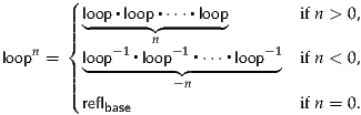
Defining a function g : Ω(S1) →Z in the other direction is a bit trickier. Note
that the successor function succ : Z →Z is an equivalence, and hence induces
a path ua(succ) : Z = Z in the universe . Thus, the recursion principle of S1
induces a map c : S1 → by c(base) :≡Z and apc(loop) : = ua(succ).
Then we have apc : (base = base) → (Z = Z), and we can define
g(p) :≡transportX X(apc(p), 0).
With these definitions, we can even prove that g(loopn) = n for any n : Z, using the induction principle Lemma 6.10.12 for n. (We will prove something more general a little later on.) However, the other equality loopg(p) = p is significantly harder. The obvious thing to try is path induction, but path induction does not apply to loops such as p : (base = base) that have both endpoints fixed! A new idea is required, one which can be explained both in terms of classical homotopy theory and in terms of type theory. We begin with the former.
In classical homotopy theory, there is a standard proof of π1(S1) = Z using
universal covering spaces. Our proof can be regarded as a type-theoretic
version of this proof, with covering spaces appearing here as fibrations whose
fibers are sets. Recall that fibrations over a space B in homotopy theory
correspond to type families B → in type theory. In particular, for a
point x0 : B, the type family (x (x0 = x)) corresponds to the path
fibration Px0B → B, in which the points of Px0B are paths in B starting at
x0, and the map to B selects the other endpoint of such a path. This
total space Px0B is contractible, since we can “retract” any path to
its initial endpoint x0 — we have seen the type-theoretic version of
this as Lemma 3.11.8. Moreover, the fiber over x0 is the loop space
Ω(B, x0) — in type theory this is obvious by definition of the loop
space.
(x0 = x)) corresponds to the path
fibration Px0B → B, in which the points of Px0B are paths in B starting at
x0, and the map to B selects the other endpoint of such a path. This
total space Px0B is contractible, since we can “retract” any path to
its initial endpoint x0 — we have seen the type-theoretic version of
this as Lemma 3.11.8. Moreover, the fiber over x0 is the loop space
Ω(B, x0) — in type theory this is obvious by definition of the loop
space.
Now in classical homotopy theory, where S1 is regarded as a topological space, we may proceed as follows. Consider the “winding” map w : R →S1, which looks like a helix projecting down onto the circle (see Figure 8.1). This map w sends each point on the helix to the point on the circle that it is “sitting above”. It is a fibration, and the fiber over each point is isomorphic to the integers. If we lift the path that goes counterclockwise around the loop on the bottom, we go up one level in the helix, incrementing the integer in the fiber. Similarly, going clockwise around the loop on the bottom corresponds to going down one level in the helix, decrementing this count. This fibration is called the universal cover of the circle.
Now a basic fact in classical homotopy theory is that a map E1 → E2 of fibrations over B which is a homotopy equivalence between E1 and E2 induces a homotopy equivalence on all fibers. (We have already seen the type-theoretic version of this as well in Theorem 4.7.7.) Since R and PbaseS1 are both contractible topological spaces, they are homotopy equivalent, and thus their fibers Z and Ω(S1) over the basepoint are also homotopy equivalent.
Let us consider how we might express the preceding proof in type theory. We
have already remarked that the path fibration of S1 is represented by
the type family (x (base = x)). We have also already seen a good
candidate for the universal cover of S1: it’s none other than the type
family c : S1 → which we defined in §8.1.1! By definition, the fiber
of this family over base is Z, while the effect of transporting around
loop is to add one — thus it behaves just as we would expect from
Figure 8.1.
(base = x)). We have also already seen a good
candidate for the universal cover of S1: it’s none other than the type
family c : S1 → which we defined in §8.1.1! By definition, the fiber
of this family over base is Z, while the effect of transporting around
loop is to add one — thus it behaves just as we would expect from
Figure 8.1.
However, since we don’t know yet that this family behaves like a universal cover is supposed to (for instance, that its total space is simply connected), we use a different name for it. For reference, therefore, we repeat the definition.
Definition 8.1.1 (Universal Cover of S1). Define code : S1 → by
circle-recursion, with
| code(base) | :≡Z | ||
| apcode(loop) | : = ua(succ). |
We emphasize briefly the definition of this family, since it is so
different from how one usually defines covering spaces in classical
homotopy theory. To define a function by circle recursion, we need to
find a point and a loop in the codomain. In this case, the codomain is
, and the point we choose is Z, corresponding to our expectation
that the fiber of the universal cover should be the integers. The loop
we choose is the successor/predecessor isomorphism on Z, which
corresponds to the fact that going around the loop in the base goes up one
level on the helix. Univalence is necessary for this part of the proof,
because we need to convert a non-trivial equivalence on Z into an
identity.
We call this the fibration of “codes”, because its elements are combinatorial data that act as codes for paths on the circle: the integer n codes for the path which loops around the circle n times.
From this definition, it is simple to calculate that transporting with code takes loop to the successor function, and loop-1 to the predecessor function:
Proof. For the first equation, we calculate as follows:
| transportcode(loop, x) | = transportA A((code A((code ), x) ), x) | (by Lemma 2.3.10) |
= transportA A(ua(succ), x) A(ua(succ), x) | (by computation for rec S1 ) | |
| = x + 1. | (by computation for ua ) |
We can now see what was wrong with our first approach: we defined f and g only on the fibers Ω(S1) and Z, when we should have defined a whole morphism of fibrations over S1. In type theory, this means we should have defined functions having types
| ∏ x:S1 | ((base = x) →code(x)) and/or | (8.1.3) |
| ∏ x:S1 | (code(x) → (base = x)) | (8.1.4) |
At this point, there are two ways to finish the proof. We can continue mimicking the classical argument by constructing (8.1.3) or (8.1.4) (it doesn’t matter which), proving that a homotopy equivalence between total spaces induces an equivalence on fibers, and then that the total space of the universal cover is contractible. The first type-theoretic proof of Ω(S1) = Z followed this pattern; we call it the homotopy-theoretic proof.
Later, however, we discovered that there is an alternative proof, which has a more type-theoretic feel and more closely follows the proofs in §§2.12 and 2.13. In this proof, we directly construct both (8.1.3) and (8.1.4), and prove that they are mutually inverse by calculation. We will call this the encode-decode proof, because we call the functions (8.1.3) and (8.1.4) encode and decode respectively. Both proofs use the same construction of the cover given above. Where the classical proof induces an equivalence on fibers from an equivalence between total spaces, the encode-decode proof constructs the inverse map (decode) explicitly as a map between fibers. And where the classical proof uses contractibility, the encode-decode proof uses path induction, circle induction, and integer induction. These are the same tools used to prove contractibility—indeed, path induction is essentially contractibility of the path fibration composed with transport—but they are applied in a different way.
Since this is a book about homotopy type theory, we present the encode-decode proof first. A homotopy theorist who gets lost is encouraged to skip to the homotopy-theoretic proof (§8.1.5).
We begin with the function (8.1.3) that maps paths to codes:
Definition 8.1.5. Define encode : ∏(x:S1) (base = x) →code(x) by
(we leave the argument x implicit).
Encode is defined by lifting a path into the universal cover, which determines an equivalence, and then applying the resulting equivalence to 0. The interesting thing about this function is that it computes a concrete number from a loop on the circle, when this loop is represented using the abstract groupoidal framework of homotopy type theory. To gain an intuition for how it does this, observe that by the above lemmas, transportcode(loop, x) is the successor map and transportcode(loop-1, x) is the predecessor map. Further, transport is functorial (Chapter 2), so transportcode(loop ▪loop, –) is

and so on. Thus, when p is a composition like

transportcode(p, –) will compute a composition of functions like

Applying this composition of functions to 0 will compute the winding number of the path—how many times it goes around the circle, with orientation marked by whether it is positive or negative, after inverses have been canceled. Thus, the computational behavior of encode follows from the reduction rules for higher-inductive types and univalence, and the action of transport on compositions and inverses.
Note that the instance encode′:≡encodebase has type (base = base) →Z. This will be one half of our desired equivalence; indeed, it is exactly the function g defined in §8.1.1.
Similarly, the function (8.1.4) is a generalization of the function loop– from §8.1.1.
Definition 8.1.6. Define decode : ∏(x:S1) code(x) → (base = x) by circle induction on x. It suffices to give a function code(base) → (base = base), for which we use loop– , and to show that loop– respects the loop.
Proof. To show that loop– respects the loop, it suffices to give a path from loop– to itself that lies over loop. By the definition of dependent paths, this means a path from

to loop– . We define such a path as follows:
transport(x′ code(x′)→(base=x′))(loop, loop– ) code(x′)→(base=x′))(loop, loop– ) | |||
= transportx′ (base=x′)(loop) ∘loop– ∘transportcode(loop-1) (base=x′)(loop) ∘loop– ∘transportcode(loop-1) | |||
| = (-▪loop) ∘ (loop– ) ∘transportcode(loop-1) | |||
| = (-▪loop) ∘ (loop– ) ∘pred | |||
= (n loopn-1 ▪loop). loopn-1 ▪loop). |
 base = x, which is post-composition of paths. On the third line, we use
the action of code on loop-1 from Lemma 8.1.2. And on the fourth line, we
simply reduce the function composition. Thus, it suffices to show that for all
n, loopn-1 ▪loop = loopn. This is an easy application of Lemma 6.10.12, using
the groupoid laws. __
base = x, which is post-composition of paths. On the third line, we use
the action of code on loop-1 from Lemma 8.1.2. And on the fourth line, we
simply reduce the function composition. Thus, it suffices to show that for all
n, loopn-1 ▪loop = loopn. This is an easy application of Lemma 6.10.12, using
the groupoid laws. __
We can now show that encode and decode are quasi-inverses. What used to be the difficult direction is now easy!
Proof. By path induction, it suffices to show that
 |
But
 |
and decodebase(0) ≡loop0 ≡reflbase. __
The other direction is not much harder.
Proof. The proof is by circle induction. It suffices to show the case for base, because the case for loop is a path between paths in Z, which is immediate because Z is a set.
Thus, it suffices to show, for all n : Z, that
The proof is by induction, using Lemma 6.10.12.
| encode′(loopn+1) | = encode′(loopn ▪loop) | (by definition of loop – ) |
| = transportcode((loopn ▪loop), 0) | (by definition of encode ) | |
| = transportcode(loop, (transportcode(loopn, 0))) | (by functoriality) | |
| = (transportcode(loopn, 0)) + 1 | (by Lemma 8.1.2) | |
| = n + 1. | (by the inductive hypothesis) |
Finally, we conclude the theorem.
Instantiating at base gives
A simple induction shows that this equivalence takes addition to composition, so that Ω(S1) = Z as groups.
Proof. For n = 1, we sketched the proof from Corollary 8.1.10 above. For
n > 1, we have  0 =
0 =  0 =
0 =  0. And
since Z is a set, Ωn-1(Z) is contractible, so this is trivial. __
0. And
since Z is a set, Ωn-1(Z) is contractible, so this is trivial. __
In §8.1.3, we defined the putative universal cover code : S1 → in type
theory, and in §8.1.5 we defined a map encode : ∏(x:S1) (base = x) →code(x)
from the path fibration to the universal cover. What remains for the classical
proof is to show that this map induces an equivalence on total spaces because
both are contractible, and to deduce from this that it must be an equivalence
on each fiber.
In Lemma 3.11.8 we saw that the total space ∑(x:S1) (base = x) is contractible. For the other, we have:
Proof. We apply the flattening lemma (Lemma 6.12.2) with the following values:
is constant at Z.
Then the type family P : S1 → defined in the flattening lemma is equivalent to
code : S1 →. Thus, the flattening lemma tells us that ∑(x:S1) code(x) is
equivalent to a higher inductive type with the following generators, which we
denote R:
We might call this type the homotopical reals; it plays the same role as the topological space R in the classical proof.
Thus, it remains to show that R is contractible. As center of contraction we choose c(0); we must now show that x = c(0) for all x : R. We do this by induction on R. Firstly, when x is c(z), we must give a path qz : c(0) = c(z), which we can do by induction on z : Z, using Lemma 6.10.12:
| q0 | : = reflc(0) | ||||||
| qn+1 | : = qn ▪pn | for n ≥ 0 | |||||
| qn-1 | : = qn ▪pn-1-1 | for n ≤ 0. |
Proof. Both types are contractible. __
Proof. Apply Theorem 4.7.7 to encode, using Corollary 8.1.13. __
In essence, the two proofs are not very different: the encode-decode one may be seen as a “reduction” or “unpackaging” of the homotopy-theoretic one. Each has its advantages; the interplay between the two points of view is part of the interest of the subject.
Note that the fibration code : S1 → together with 0 : code(base) is a pointed
predicate in the sense of Definition 5.8.1. From this point of view, we can see
that the encode-decode proof in §8.1.4 consists of proving that code satisfies
Theorem 5.8.2(iii), while the homotopy-theoretic proof in §8.1.5 consists
of proving that it satisfies Theorem 5.8.2(iv). This suggests a third
approach.
Theorem 8.1.15. The pair (code, 0) is an identity system at base : S1 in the sense of Definition 5.8.1.
Proof. Let D : ∏(x:S1) code(x) → and d : D(base, 0) be given; we want
to define a function f : ∏(x:S1) ∏(c:code(x)) D(x, c). By circle induction,
it suffices to specify f(base) : ∏(c:code(base)) D(base, c) and verify that
loop
* = f(base).
Of course, code(base) ≡ Z. By Lemma 8.1.2 and induction on n,
we may obtain a path pn : transportcode(loopn, 0) = n for any integer
n. Therefore, by paths in Σ-types, we have a path pair=(loopn, pn) :
(base, 0) = (base, n) in ∑(x:S1) code(x). Transporting d along this path
in the fibration  : ( ∑(x:S1) code(x)) → associated to D, we obtain
an element of D(base, n) for any n : Z. We define this element to be
f(base)(n):
: ( ∑(x:S1) code(x)) → associated to D, we obtain
an element of D(base, n) for any n : Z. We define this element to be
f(base)(n):

Now we need transportλx. ∏(c:code(x)) D(x,c)(loop, f(base)) = f(base). By Lemma 2.9.7, this means we need to show that for any n : Z,
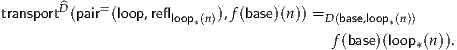
 = n + 1, so transporting along this, it
suffices to show
= n + 1, so transporting along this, it
suffices to show 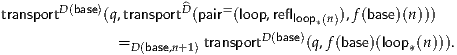 |

However, expanding out the definition of f(base), we have
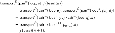
This completes the construction of f : ∏(x:S1) ∏(c:code(x)) D(x, c). Since

we have shown that (code, 0) is an identity system. __
Proof. By Theorem 5.8.2. __
Of course, this proof also contains essentially the same elements as the previous two. Roughly, we can say that it unifies the proofs of Definition 8.1.6 and Lemma 8.1.8, performing the requisite inductive argument only once in a generic case.
Recall from §7.5 that a type A is called n-connected if  n is contractible.
The aim of this section is to prove that the operation of suspension from §6.5
increases connectedness.
n is contractible.
The aim of this section is to prove that the operation of suspension from §6.5
increases connectedness.
Proof. We remarked in §6.8 that the suspension of A is the pushout 1 ⊔A1, so we need to prove that the following type is contractible:

By Theorem 7.4.12 we know that  n+1 is a pushout in
(n + 1)-Type of the diagram
n+1 is a pushout in
(n + 1)-Type of the diagram
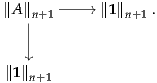
Given that  n+1 = 1, the type
  n+1 is also a pushout of the
following diagram in (n + 1)-Type (because both diagrams are equal)
n+1 is also a pushout of the
following diagram in (n + 1)-Type (because both diagrams are equal)
We will now prove that 1 is also a pushout of in (n + 1)-Type. Let E
be an (n + 1)-truncated type; we need to prove that the following map is
an equivalence
where we recall that cocone (E) is the type
The map  is an equivalence, hence we also
have
is an equivalence, hence we also
have
Now A is n-connected hence so is  n+1 because
  n =
n =
 n = 1, and (x = Ey) is n-truncated because E is (n + 1)-connected.
Hence by Corollary 7.5.9 the following map is an equivalence
n = 1, and (x = Ey) is n-truncated because E is (n + 1)-connected.
Hence by Corollary 7.5.9 the following map is an equivalence
Hence we have
But the following map is an equivalence
Hence
Finally we get an equivalence
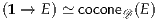
We can now unfold the definitions in order to get the explicit expression of this map, and we see easily that this is exactly the map we had at the beginning.
Hence we proved that 1 is a pushout of in (n + 1)-Type. Using
uniqueness of pushouts we get that  n+1 = 1 which proves that
the suspension of A is (n + 1)-connected. __
n+1 = 1 which proves that
the suspension of A is (n + 1)-connected. __
Proof. We prove this by induction on n. For n = 0 we have to prove that S0 is merely inhabited, which is clear. Let n : N be such that Sn is (n- 1)-connected. By definition Sn+1 is the suspension of Sn, hence by the previous lemma Sn+1 is n-connected. __
Let (A, a) be a pointed type and n : N. Recall from Example 6.11.4 that if n > 0 the set πn(A, a) has a group structure, and if n > 1 the group is abelian.
We can now say something about homotopy groups of n-truncated and n-connected types.
Proof. The loop space of an n-type is an (n- 1)-type, hence Ωk(A, a)
is an (n-k)-type, and we have (n-k) ≤ -1 so Ωk(A, a) is a mere
proposition. But Ωk(A, a) is inhabited, so it is actually contractible and
πk(A, a) =  0 =
0 =  0 = 1. __
Proof. We have the following sequence of equalities:
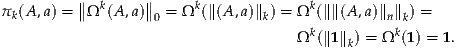
Proof. The sphere Sn is (n- 1)-connected by Corollary 8.2.2, so we can apply Lemma 8.3.2. __
If the codomain of a function f : X → Y is equipped with a basepoint y0 : Y, then we refer to the fiber F :≡fibf(y0) of f over y0 as the fiber of f. (If Y is connected, then F is determined up to mere equivalence; see Exercise 8.5.) We now show that if X is also pointed and f preserves basepoints, then there is a relation between the homotopy groups of F, X, and Y in the form of a long exact sequence. We derive this by way of the fiber sequence associated to such an f.
Definition 8.4.1. A pointed map between pointed types (X, x0) and (Y, y0) is a map f : X → Y together with a path f0 : f(x0) = y0.
For any pointed types (X, x0) and (Y, y0), there is a pointed map (λx.y0) : X → Y which is constant at the basepoint. We call this the zero map and sometimes write it as 0 : X → Y.
Recall that every pointed type (X, x0) has a loop space Ω(X, x0). We now note that this operation is functorial on pointed maps.
Definition 8.4.2. Given a pointed map between pointed types f : X → Y, we define a pointed map Ωf : ΩX → ΩY by
The path (Ωf)0 : (Ωf)(reflx0) = refly0, which exhibits Ωf as a pointed map, is the obvious path of type
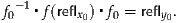
There is another functor on pointed maps, which takes f : X → Y to pr1 : fibf(y0) → X. When f is pointed, we always consider fibf(y0) to be pointed with basepoint (x0, f0), in which case pr1 is also a pointed map, with witness (pr1)0 :≡reflx0. Thus, this operation can be iterated.
Definition 8.4.3. The fiber sequence of a pointed map f : X → Y is the infinite sequence of pointed types and pointed maps

defined recursively by

and
| X(n+1) | :≡fibf(n-1)(x0(n-1)) | |||||
| f(n) | :≡pr1 | : X(n+1) → X(n). |
Thus, any adjacent pair of maps in this fiber sequence is of the form

In particular, we have f(n-1) ∘f(n) = 0. We now observe that the types occurring in this sequence are the iterated loop spaces of the base space Y, the total space X, and the fiber F :≡fibf(y0), and similarly for the maps.
Proof. For (i), we have
| fib f(1)(x0) | :≡ ∑ z:fibf(y0) (pr1(z) = x0) | |||||
| ≃ ∑ (x:A) ∑ (p:f(x)=y0) (x = x0) | (by Exercise 2.10) | |||||
| ≃ (f(x0) = y0) | (as ∑(x:A) (x = x0) is contractible) | |||||
| ≃ (y0 = y0) | (by (f0 ▪ –)) | |||||
| ≡ ΩY. |
 ▪p,
while its inverse sends r : y0 = y0 to ((x0, f0 ▪r), reflx0). In particular, the
basepoint ((x0, f0), reflx0) of fibf(1)(x0) is sent to f0-1 ▪f
▪p,
while its inverse sends r : y0 = y0 to ((x0, f0 ▪r), reflx0). In particular, the
basepoint ((x0, f0), reflx0) of fibf(1)(x0) is sent to f0-1 ▪f ▪f0,
which equals refly0. Hence this equivalence is a pointed map (see
Exercise 8.7). Moreover, under this equivalence, f(2) is identified with
λr.(x0, f0 ▪r) : ΩY →fibf(y0).
▪f0,
which equals refly0. Hence this equivalence is a pointed map (see
Exercise 8.7). Moreover, under this equivalence, f(2) is identified with
λr.(x0, f0 ▪r) : ΩY →fibf(y0).
Item (ii) follows immediately by applying (i) to f(1) in place of f.
Since (f(1))0 :≡reflx0, under this equivalence f(3) is identified with
the map ΩX →fibf(1)(x0) defined by s ((x0, f0), s). Thus, when
we compose with the previous equivalence fibf(1)(x0) ≃ ΩY, we see
that s maps to f0-1 ▪f
((x0, f0), s). Thus, when
we compose with the previous equivalence fibf(1)(x0) ≃ ΩY, we see
that s maps to f0-1 ▪f ▪f
0, which is by definition (Ωf)(s-1),
giving (iii). __
▪f
0, which is by definition (Ωf)(s-1),
giving (iii). __
Thus, the fiber sequence of f : X → Y can be pictured as:

where the minus signs denote composition with path inversion (–)-1. Note that by Exercise 8.6, we have

Thus, there are minus signs on the k-fold loop maps whenever k is odd.
From this fiber sequence we will deduce an exact sequence of pointed sets. Let A and B be sets and f : A → B a function, and recall from Definition 7.6.3 the definition of the image im(f), which can be regarded as a subset of B:

If A and B are moreover pointed with basepoints a0 and b0, and f is a pointed map, we define the kernel of f to be the following subset of A:
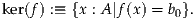
Of course, this is just the fiber of f over the basepoint b0; it a subset of A because B is a set.
Note that any group is a pointed set, with its unit element as basepoint, and any group homomorphism is a pointed map. In this case, the kernel and image agree with the usual notions from group theory.
Definition 8.4.5. An exact sequence of pointed sets is a (possibly bounded) sequence of pointed sets and pointed maps:

such that for every n, the image of f(n) is equal, as a subset of A(n), to the kernel of f(n-1). In other words, for all a : A(n) we have

where a0(n) denotes the basepoint of A(n).
Usually, most or all of the pointed sets in an exact sequence are groups, and often abelian groups. When we speak of an exact sequence of groups, it is assumed moreover that the maps are group homomorphisms and not just pointed maps.
Theorem 8.4.6. Let f : X → Y be a pointed map between pointed spaces with fiber F :≡ fibf(y0). Then we have the following long exact sequence, which consists of groups except for the last three terms, and abelian groups except for the last six.
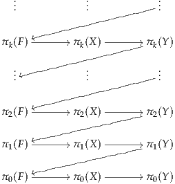
Proof. We begin by showing that the 0-truncation of a fiber sequence is an exact sequence of pointed sets. Thus, we need to show that for any adjacent pair of maps in a fiber sequence:
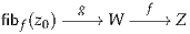
with g :≡pr1, the sequence
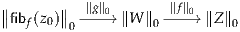
is exact, i.e. that im( 0) ⊆ ker(
 0) and ker(
 0) ⊆im(
 0).
0).
The first inclusion is equivalent to  0 ∘
0 ∘ 0 = 0, which holds
by functoriality of ∥–∥0 and the fact that g ∘f = 0. For the second,
we assume w′ :
0 = 0, which holds
by functoriality of ∥–∥0 and the fact that g ∘f = 0. For the second,
we assume w′ :  0 and p′ :
  0(w′) =
  0 and show there
merely exists t : fibf(z0) such that g(t) = w′. Since our goal is a
mere proposition, we can assume that w′ is of the form
0 and show there
merely exists t : fibf(z0) such that g(t) = w′. Since our goal is a
mere proposition, we can assume that w′ is of the form  0 for some
w : W. Now by Theorem 7.3.12, p′ :
0 for some
w : W. Now by Theorem 7.3.12, p′ :  0 =
0 =  0 yields p′′ :
 -1, so by a further truncation induction we may assume
some p : f(w) = z0. But now we have
-1, so by a further truncation induction we may assume
some p : f(w) = z0. But now we have  0 :
0 :  0 whose
image under
0 whose
image under  0 is
0 is  0 ≡ w′, as desired.
Thus, applying ∥–∥0 to the fiber sequence of f, we obtain a long exact sequence involving the pointed sets πk(F), πk(X), and πk(Y) in the desired order. And of course, πk is a group for k ≥ 1, being the 0-truncation of a loop space, and an abelian group for k ≥ 2 by the Eckmann–Hilton argument (Theorem 2.1.6). Moreover, Lemma 8.4.4 allows us to identify the maps πk(F) → πk(X) and πk(X) → πk(Y) in this exact sequence as (-1)kπk(i) and (-1)kπk(f) respectively.
More generally, every map in this long exact sequence except the
last three is of the form  0 or
0 or  0 for some h. In the
former case it is a group homomorphism, while in the latter case
it is a homomorphism if the groups are abelian; otherwise it is an
“anti-homomorphism”. However, the kernel and image of a group
homomorphism are unchanged when we replace it by its negative, and
hence so is the exactness of any sequence involving it. Thus, we can
modify our long exact sequence to obtain one involving πk(i) and πk(f)
directly and in which all the maps are group homomorphisms (except
the last three). __
0 for some h. In the
former case it is a group homomorphism, while in the latter case
it is a homomorphism if the groups are abelian; otherwise it is an
“anti-homomorphism”. However, the kernel and image of a group
homomorphism are unchanged when we replace it by its negative, and
hence so is the exactness of any sequence involving it. Thus, we can
modify our long exact sequence to obtain one involving πk(i) and πk(f)
directly and in which all the maps are group homomorphisms (except
the last three). __
The usual properties of exact sequences of abelian groups can be proved as usual. In particular we have:
Proof. Since the kernel of f is the image of K → G, if K = 0 then the kernel of f is {0}; hence f is injective because it’s a group morphism. Similarly, since the image of f is the kernel of H → Q, if Q = 0 then the image of f is all of H, so f is surjective. Finally, (iii) follows from (i) and (ii) by Theorem 4.6.3. __
As an immediate application, we can now quantify in what way n-connectedness of a map is stronger than inducing an equivalence on n-truncations.
Corollary 8.4.8. Let f : A → B be n-connected and a : A, and define b :≡ f(a). Then:
Proof. As part of the long exact sequence, for each k we have an exact sequence

Now since f is n-connected,  n is contractible. Therefore,
if k ≤ n, then πk(fibf(b)) =
n is contractible. Therefore,
if k ≤ n, then πk(fibf(b)) =  0 = Ωk(
 k)
is also contractible. Thus, πk(f) is an isomorphism for k ≤ n
by Lemma 8.4.7(iii), while for k = n + 1 it is surjective by
Lemma 8.4.7(ii). __
k)
is also contractible. Thus, πk(f) is an isomorphism for k ≤ n
by Lemma 8.4.7(iii), while for k = n + 1 it is surjective by
Lemma 8.4.7(ii). __
In §8.8 we will see that the converse of Corollary 8.4.8 also holds.
In this section we will define the Hopf fibration.
Theorem 8.5.1 (Hopf Fibration). There is a fibration H over S2 whose fiber over the basepoint is S1 and whose total space is S3.
The Hopf fibration will allow us to compute several homotopy groups of spheres. Indeed, it yields the following long exact sequence of homotopy groups (see §8.4):
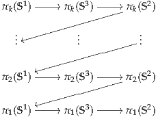
We’ve already computed all πn(S1), and πk(Sn) for k < n, so this becomes the following:
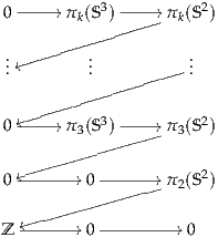
In particular we get the following result:
Corollary 8.5.2. We have π2(S2) ≃Z and πk(S3) ≃ πk(S2) for every k ≥ 3 (where the map is induced by the Hopf fibration, seen as a map from the total space S3 to the base space S2).
In fact, we can say more: the fiber sequence of the Hopf fibration will show that Ω3(S3) is the fiber of a map from Ω3(S2) to Ω2(S1). Since Ω2(S1) is contractible, we have Ω3(S3) ≃ Ω3(S2). In classical homotopy theory, this fact would be a consequence of Corollary 8.5.2 and Whitehead’s theorem, but Whitehead’s theorem is not necessarily valid in homotopy type theory (see §8.8). We will not use the more precise version here though.
We first start with a lemma explaining how to construct fibrations over pushouts.
Lemma 8.5.3. Let = (Y
 ) be a span and assume that we have
and EZ : Z →.
and EZ ∘k : X →, i.e.
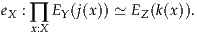
Then we can construct a fibration E : Y ⊔XZ →such that
 = ua(eX(x)) (note that both sides of the
equation are paths in from EY(j(x)) to EZ(k(x))).
= ua(eX(x)) (note that both sides of the
equation are paths in from EY(j(x)) to EZ(k(x))).Moreover, the total space of this fibration fits in the following pushout square:
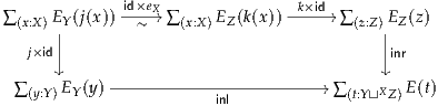
Proof. We define E by the recursion principle of the pushout Y ⊔XZ. For that, we need to specify the value of E on elements of the form inl(y), inr(z) and the action of E on paths glue(x), so we can just choose the following values:
| E(inl(y)) | :≡ EY(y), | ||
| E(inr(z)) | :≡ EZ(z), | ||
E | : = ua(eX(x)). |
is defined by
 |
The base higher inductive type W in the flattening lemma is equivalent to the
pushout Y ⊔XZ and the type family P : Y ⊔XZ → is equivalent to the E
defined above.
Thus the flattening lemma tells us that ∑(t:Y⊔XZ) E(t) is equivalent the higher inductive type Etot′ with the following generators:
 |
Using the flattening lemma again or a direct computation, it is easy to see that ∑ (a:Y+Z) C(a) ≃ ∑(y:Y) EY(y) + ∑(z:Z) EZ(z), hence Etot′ is equivalent to the higher inductive type Etot with the following generators:
 |
Thus the total space of E is the pushout of the total spaces of EY and EZ, as required. __
Definition 8.5.4. An H-space consists of
Lemma 8.5.5. Let A be a connected H-space. Then for every a : A, the maps μ(a, –) : A → Aand μ(–, a) : A → Aare equivalences.
Proof. Let us prove that for every a : A the map μ(a, –) is an equivalence. The other statement is symmetric. The statement that μ(a, –) is an equivalence corresponds to a type family P : A →Prop and proving it corresponds to finding a section of this type family.
The type Prop is a set (Theorem 7.1.11) hence we can define a new
type family P′ :  0 →Prop by P′(
 0) :≡ P(a). But A is connected
by assumption, hence
0) :≡ P(a). But A is connected
by assumption, hence  0 is contractible. This implies that in order to
find a section of P′, it is enough to find a point in the fiber of P′ over
0 is contractible. This implies that in order to
find a section of P′, it is enough to find a point in the fiber of P′ over  0.
But we have P′(
0.
But we have P′( 0) = P(e) which is inhabited because μ(e, –) is equal
to the identity map by definition of an H-space, hence is an equivalence.
0) = P(e) which is inhabited because μ(e, –) is equal
to the identity map by definition of an H-space, hence is an equivalence.
We have proved that for every x :  0 the proposition P′(x) is true,
hence in particular for every a : A the proposition P(a) is true because
P(a) is P′(
0 the proposition P′(x) is true,
hence in particular for every a : A the proposition P(a) is true because
P(a) is P′( 0). __
Definition 8.5.6. Let A be a connected H-space. We define a fibration over ΣA using Lemma 8.5.3.
Given that ΣA is the pushout 1⊔A1, we can define a fibration over ΣA by specifying
We take A for F1 and F2, and for a : A we take the equivalence μ(a, –) for e(a).
According to Lemma 8.5.3, we have the following diagram:
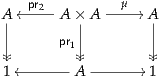
and the fibration we just constructed is a fibration over ΣA whose total space is the pushout of the top line.
Moreover, with f(x, y) :≡ (μ(x, y), y) we have the following diagram:
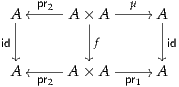
The diagram commutes and the three vertical maps are equivalences, the inverse of f being the function g defined by
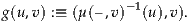
This shows that the two lines are equivalent (hence equal) spans, so the total space of the fibration we constructed is equivalent to the pushout of the bottom line. And by definition, this latter pushout is the join of A with itself (see §6.8). We have proven:
Lemma 8.5.7. Given a connected H-space A, there is a fibration, called the Hopf construction, over ΣAwith fiber Aand total space A*A.
We will first construct a structure of H-space on the circle S1, hence by Lemma 8.5.7 we will get a fibration over S2 with fiber S1 and total space S1 *S1. We will then prove that this join is equivalent to S3.
Proof. For the base point of the H-space structure we choose base. Now
we need to define the multiplication operation μ : S1 ×S1 →S1. We
will define the curried form  : S1 → (S1 →S1) of μ by recursion on
S1:
: S1 → (S1 →S1) of μ by recursion on
S1:
 |
where h : ∏(x:S1) (x = x) is the function defined in Lemma 6.4.2, which has the property that h(base) :≡loop.
Now we just have to prove that μ(x, base) = μ(base, x) = x for every x : S1.
By definition, if x : S1 we have μ(base, x) =  (base)(x) = idS1(x) = x. For the
equality μ(x, base) = x we do it by induction on x : S1:
(base)(x) = idS1(x) = x. For the
equality μ(x, base) = x we do it by induction on x : S1:

The left-hand side is equal to loop, and for the right-hand side we have:
| apλx.μ(x,base)(loop) ▪reflbase | = apλx.( (x))(base)(loop) (x))(base)(loop) | ||
= happly(apλx.( (x))(loop), base) (x))(loop), base) | |||
| = happly(funext(h), base) | |||
| = h(base) | |||
| = loop. | __
Now recall from §6.8 that the join A*B of types A and B is the pushout of the diagram
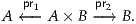
Lemma 8.5.9. The operation of join is associative: if A, Band C are three types then we have an equivalence (A*B) *C ≃ A* (B*C).
Proof. We define a map f : (A*B) *C → A* (B*C) by induction. We first need to define f ∘inl : A*B → A* (B*C) which will be done by induction, then f ∘inr : C → A* (B*C), and then apf ∘glue : ∏(t:(A*B)×C) f(inl(pr1(t))) = f(inr(pr2(t))) which will be done by induction on the first component of t:
| (f ∘inl)(inl(a))) | :≡inl(a), | ||
| (f ∘inl)(inr(b))) | :≡inr(inl(b)), | ||
| apf∘inl(glue(a, b)) | : = glue(a, inl(b)), | ||
| f(inr(c)) | :≡inr(inr(c)), | ||
| apf(glue(inl(a), c)) | : = glue(a, inr(c)), | ||
| apf(glue(inr(b), c)) | : = apinr(glue(b, c)), | ||
| apdλx.apf(glue(x,c))(glue(a, b)) | : = “apdλx.glue(a,x)(glue(b, c))′′. |

whereas it is supposed to be of type
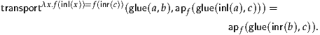

and so we can coerce by an equivalence to obtain the necessary element. Similarly, we can define a map g : A* (B*C) → (A*B) *C, and checking that f and g are inverse to each other is a long and tedious but essentially straightforward computation. __
A more conceptual proof sketch is as follows.
Proof. Let us consider the following diagram where the maps are the obvious projections:
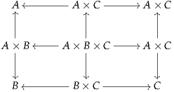
Taking the colimit of the columns gives the following diagram, whose colimit is (A*B) *C:

On the other hand, taking the colimit of the lines gives a diagram whose colimit is A* (B*C).
Hence using a Fubini-like theorem for colimits (that we haven’t proved) we have an equivalence (A*B) *C ≃ A* (B*C). The proof of this Fubini theorem for colimits still requires the long and tedious computation, though. __
Proof. It is easy to define the two maps back and forth and to prove that they are inverse to each other. The details are left as an exercise to the reader. __
We can now construct the Hopf fibration:
Proof. We proved that S1 has a structure of H-space (cf Lemma 8.5.8) hence by Lemma 8.5.7 there is a fibration over S2 of fiber S1 and total space S1 *S1. But by the two previous results and Lemma 6.5.1 we have:
 |
Before proving the Freudenthal suspension theorem, we need some auxiliary lemmas about connectedness. In Chapter 7 we proved a number of facts about n-connected maps and n-types for fixed n; here we are now interested in what happens when we vary n. For instance, in Lemma 7.5.7 we showed that n-connected maps are characterized by an “induction principle” relative to families of n-types. If we want to “induct along” an n-connected map into a family of k-types for k > n, we don’t immediately know that there is a function by such an induction principle, but the following lemma says that at least our ignorance can be quantified.
Lemma 8.6.1. If f : A → B is n-connected and P : B → k-Type is a family of k-types for k ≥ n, then the induced function
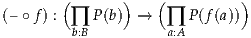
is (k-n- 2)-truncated.
Proof. We induct on the natural number k- n. When k = n, this is Lemma 7.5.7. For the inductive step, suppose f is n-connected and P is a family of (k + 1)-types. To show that (– ∘f) is (k-n- 1)-truncated, let ℓ : ∏(a:A) P(f(a)); then we have
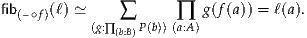
Let (g, p) and (h, q) lie in this type, so p : g∘f ~ ℓ and q : h∘f ~ ℓ; then we also have
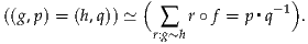
However, here the right-hand side is a fiber of the map
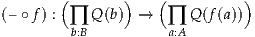
where Q(b) :≡ (g(b) = h(b)). Since P is a family of (k + 1)-types, Q is a family of k-types, so the inductive hypothesis implies that this fiber is a (k-n- 2)-type. Thus, all path spaces of fib(–∘f)(ℓ) are (k-n- 2)-types, so it is a (k-n- 1)-type. __
Recall that if (A, a0) and (B, b0) are pointed types, then their wedge A∨B
is defined to be the pushout of A
 . There is a canonical map
i : A∨B → A×B defined by the two maps λa.(a, b0) and λb.(a0, b); the
following lemma essentially says that this map is highly connected if A and B
are so. It is a bit more convenient both to prove and use, however, if
we use the characterization of connectedness from Lemma 7.5.7 and
substitute in the universal property of the wedge (generalized to type
families).
. There is a canonical map
i : A∨B → A×B defined by the two maps λa.(a, b0) and λb.(a0, b); the
following lemma essentially says that this map is highly connected if A and B
are so. It is a bit more convenient both to prove and use, however, if
we use the characterization of connectedness from Lemma 7.5.7 and
substitute in the universal property of the wedge (generalized to type
families).
Lemma 8.6.2 (Wedge connectivity lemma). Suppose that (A, a0) and (B, b0) are n- and m-connected pointed types, respectively, with n, m ≥ 0, and let
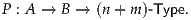 |
Then for any f : ∏(a:A) P(a, b0) and g : ∏(b:B) P(a0, b) with p : f(a0) = g(b0), there exists h : ∏(a:A) ∏(b:B) P(a, b) with homotopies
 |
such that p = q(a0)-1 ▪r(b 0).
Proof. Define P : A → by
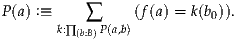
Then we have (g, p) : P(a0). Since a0 : 1 → A is (n- 1)-connected, if P is a family of (n- 1)-types then we will have ℓ : ∏(a:A) P(a) such that ℓ(a0) = (g, p), in which case we can define h(a, b) :≡pr1(ℓ(a))(b). However, for fixed a, the type P(a) is the fiber over f(a) of the map
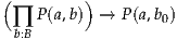
given by precomposition with b0 : 1 → B. Since b0 : 1 → B is (m- 1)-connected, for this fiber to be (n- 1)-truncated, by Lemma 8.6.1 it suffices for each type P(a, b) to be an (n + m)-type, which we have assumed. __
Let (X, x0) be a pointed type, and recall the definition of the suspension ΣX from §6.5, with constructors N, S : ΣX and merid : X → (N = S). We regard ΣX as a pointed space with basepoint N, so that we have ΩΣX :≡ (N =ΣX N). Then there is a canonical map
| σ | : X → ΩΣX | ||
| σ(x) | :≡merid(x) ▪merid(x0)-1. |
Remark 8.6.3. In classical algebraic topology, one considers the reduced suspension, in which the path merid(x0) is collapsed down to a point, identifying N and S. The reduced and unreduced suspensions are homotopy equivalent, so the distinction is invisible to our purely homotopy-theoretic eyes — and higher inductive types only allow us to “identify” points up to a higher path anyway, there is no purpose to considering reduced suspensions in homotopy type theory. However, the “unreducedness” of our suspension is the reason for the (possibly unexpected) appearance of merid(x0)-1 in the definition of σ.
Our goal is now to prove the following.
Theorem 8.6.4 (The Freudenthal suspension theorem). Suppose that X is n-connected and pointed, with n ≥ 0. Then the map σ : X → ΩΣ(X) is 2n-connected.
We will use the encode-decode method, but applied in a slightly different
way. In most cases so far, we have used it to characterize the loop space
Ω(A, a0) of some type as equivalent to some other type B, by constructing a
family code : A → with code(a0) :≡ B and a family of equivalences
decode : ∏(x:A) code(x) ≃ (a0 = x).
In this case, however, we want to show that σ : X → ΩΣX is 2n-connected.
We could use a truncated version of the previous method, such as we will see
in §8.7, to prove that  2n →
2n → 2n is an equivalence—but this is
a slightly weaker statement than the map being 2n-connected (see
Corollaries 8.4.8 and 8.8.5). However, note that in the general case,
to prove that decode(x) is an equivalence, we could equivalently be
proving that its fibers are contractible, and we would still be able to
use induction over the base type. This we can generalize to prove
connectedness of a map into a loop space, i.e. that the truncations of its fibers
are contractible. Moreover, instead of constructing code and decode
separately, we can construct directly a family of codes for the truncations of the
fibers.
2n is an equivalence—but this is
a slightly weaker statement than the map being 2n-connected (see
Corollaries 8.4.8 and 8.8.5). However, note that in the general case,
to prove that decode(x) is an equivalence, we could equivalently be
proving that its fibers are contractible, and we would still be able to
use induction over the base type. This we can generalize to prove
connectedness of a map into a loop space, i.e. that the truncations of its fibers
are contractible. Moreover, instead of constructing code and decode
separately, we can construct directly a family of codes for the truncations of the
fibers.
Definition 8.6.5. If X is n-connected and pointed with n ≥ 0, then there is a family
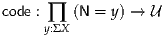 | (8.6.6) |
such that
| code(N, p) | :≡ 2n ≡ 2n ≡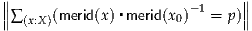 2n 2n | (8.6.7) |
| code(S, q) | :≡ 2n ≡ 2n ≡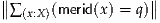 2n. 2n. | (8.6.8) |
Our eventual goal will be to prove that code(y, p) is contractible for all y : ΣX and p : N = y. Applying this with y :≡N will show that all fibers of σ are 2n-connected, and thus σ is 2n-connected.
Proof of Definition 8.6.5. We define code(y, p) by induction on y : ΣX, where the first two cases are (8.6.7) and (8.6.8). It remains to construct, for each x1 : X, a dependent path
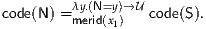
By Lemma 2.9.6, this is equivalent to giving a family of paths

And by univalence and transport in path types, this is equivalent to a family of equivalences
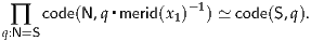
We will define a family of maps
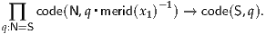 | (8.6.9) |
and then show that they are all equivalences. Thus, let q : N = S; by the universal property of truncation and the definitions of code(N, –) and code(S, –), it will suffice to define for each x2 : X, a map
 |
Now for each x1, x2 : X, this type is 2n-truncated, while X is n-connected. Thus, by Lemma 8.6.2, it suffices to define this map when x1 is x0, when x2 is x0, and check that they agree when both are x0.
When x1 is x0, the hypothesis is r : merid(x2) ▪merid(x0)-1 = q▪merid(x
0)-1.
Thus, by canceling merid(x0)-1 from r to get r′ : merid(x
2) = q, so we can
define the image to be  2n.
2n.
When x2 is x0, the hypothesis is r : merid(x0) ▪merid(x0)-1 = q▪merid(x
1)-1.
Rearranging this, we obtain r′′ : merid(x1) = q, and we can define the image
to be  2n.
2n.
Finally, when both x1 and x2 are x0, it suffices to show the resulting r′ and r′′ agree; this is an easy lemma about path composition. This completes the definition of (8.6.9). To show that it is a family of equivalences, since being an equivalence is a mere proposition and x0 : 1 → X is (at least) (-1)-connected, it suffices to assume x1 is x0. In this case, inspecting the above construction we see that it is essentially the 2n-truncation of the function that cancels merid(x0)-1, which is an equivalence. __
In addition to (8.6.7) and (8.6.8), we will need to extract from the construction of code some information about how it acts on paths. For this we use the following lemma.
Lemma 8.6.10. Let A : , B : A →, and C : ∏(a:A) B(a) →, and also
a1, a2 : Awith m : a1 = a2 and b : B(a2). Then the function

where t : transportB(m, transportB(m-1, b)) = b is the obvious coherence path and
 : ( ∑(a:A) B(a)) →is the uncurried form of C, is equal to the equivalence
obtained by univalence from the composite
: ( ∑(a:A) B(a)) →is the uncurried form of C, is equal to the equivalence
obtained by univalence from the composite
| C(a1, transportB(m-1, b)) | = transportλa.B(a)→(m, C(a1))(b) | (by (2.9.4)) |
| = C(a2, b). | (by happly (apdC , b)) , b)) |
Proof. By path induction, we may assume a2 is a1 and m is refla1, in which case both functions are the identity. __
We apply this lemma with A :≡ ΣX and B :≡ λy.(N = y) and
C :≡code, while a1 :≡N and a2 :≡S and m :≡merid(x1) for some
x1 : X, and finally b :≡ q is some path N = S. The computation rule for
induction over ΣX identifies apdC with a path constructed in a
certain way out of univalence and function extensionality. The second
function described in Lemma 8.6.10 essentially consists of undoing these
applications of univalence and function extensionality, reducing back to the
particular functions (8.6.9) that we defined using Lemma 8.6.2. Therefore,
Lemma 8.6.10 says that transporting along pair=(q, t) essentially recovers
these functions.
with a path constructed in a
certain way out of univalence and function extensionality. The second
function described in Lemma 8.6.10 essentially consists of undoing these
applications of univalence and function extensionality, reducing back to the
particular functions (8.6.9) that we defined using Lemma 8.6.2. Therefore,
Lemma 8.6.10 says that transporting along pair=(q, t) essentially recovers
these functions.
Finally, by construction, when x1 or x2 coincides with x0 and the input is in
the image of  2n, we know more explicitly what these functions are. Thus,
for any x2 : X, we have
2n, we know more explicitly what these functions are. Thus,
for any x2 : X, we have
 | (8.6.11) |
where r : merid(x2) ▪merid(x0)-1 = transportB(merid(x 0)-1, q) is arbitrary as before, and r′ : merid(x2) = q is obtained from r by identifying its end point with q▪merid(x0)-1 and canceling merid(x 0)-1. Similarly, for any x 1 : X, we have
 | (8.6.12) |
where r : merid(x0) ▪merid(x0)-1 = transportB(merid(x 1)-1, q), and r′′ : merid(x1) = q is obtained by identifying its end point and rearranging paths.
Proof of Theorem 8.6.4. It remains to show that code(y, p) is contractible for each y : ΣX and p : N = y. First we must choose a center of contraction, say c(y, p) : code(y, p). This corresponds to the definition of the function encode in our previous proofs, so we define it by transport. Note that in the special case when y is N and p is reflN, we have

Thus, we can choose c(N, reflN) :≡  2n, where rinvq
is the obvious path q ▪ q-1 = refl for any q. We can now obtain
c : ∏(y:ΣX) ∏(p:N=y) code(y, p) by path induction on p, but it will be
important below that we can also give a concrete definition in terms of
transport:
2n, where rinvq
is the obvious path q ▪ q-1 = refl for any q. We can now obtain
c : ∏(y:ΣX) ∏(p:N=y) code(y, p) by path induction on p, but it will be
important below that we can also give a concrete definition in terms of
transport:

where  :
:  ∑(y:ΣX) (N = y)
 → is the uncurried version of code,
and tidp : p*
→ is the uncurried version of code,
and tidp : p* = p is a standard lemma.
Next, we must show that every element of code(y, p) is equal to
c(y, p). Again, by path induction, it suffices to assume y is N and p is reflN.
In fact, we will prove it more generally when y is N and p is arbitrary.
That is, we will show that for any p : N = N and d : code(N, p) we have
d = c(N, p). Since this equality is a (2n- 1)-type, we may assume d is of
the form  2n for some x1 : X and r : merid(x1) ▪merid(x0)-1 = p.
Now by a further path induction, we may assume that r is reflexivity, and p is merid(x1) ▪merid(x0)-1. (This is why we generalized to arbitrary p above.) Thus, we have to prove that
 | (8.6.13) |
By definition, the right-hand side of this equality is
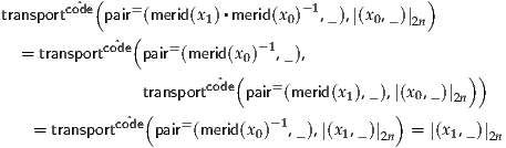 |
Corollary 8.6.14 (Freudenthal Equivalence). Suppose that X is
n-connected and pointed, with n ≥ 0. Then  2n ≃
2n ≃ 2n.
2n.
Proof. By Theorem 8.6.4, σ is 2n-connected. By Lemma 7.5.14, it is therefore an equivalence on 2n-truncations. __
One important corollary of the Freudenthal suspension theorem is that the homotopy groups of spheres are stable in a certain range (these are the northeast-to-southwest diagonals in Table 8.1):
Proof. Assume k ≤ 2n- 2. By Corollary 8.2.2, Sn is (n- 1)-connected. Therefore, by Corollary 8.6.14,
By Lemma 7.3.15, because k ≤ 2(n- 1), applying  k to both sides shows
that this equation holds for k:
k to both sides shows
that this equation holds for k:
 | (8.6.16) |
Then, the main idea of the proof is as follows; we omit checking that these equivalences act appropriately on the base points of these spaces:
| πk+1(Sn+1) | ≡ 0 0 | ||
≡ 0 0 | |||
≡ 0 0 | |||
= Ωk( k) k) | (by Theorem 7.3.12) | ||
= Ωk( k) k) | (by (8.6.16)) | ||
=  0 0 | (by Theorem 7.3.12) | ||
| ≡ πk(Sn). | __
This means that once we have calculated one entry in one of these stable diagonals, we know all of them. For example:
Proof. The proof is by induction on n. We already have π1(S1) = Z (Corollary 8.1.11) and π2(S2) = Z (Corollary 8.5.2). When n ≥ 2, n ≤ (2n- 2). Therefore, by Corollary 8.6.15, πn+1(Sn+1) = πn(Sn), and this equivalence, combined with the inductive hypothesis, gives the result. __
Proof. By Corollary 8.5.2, π3(S2) = π3(S3). But by Theorem 8.6.17, π3(S3) = Z. __
The van Kampen theorem calculates the fundamental group π1 of a (homotopy) pushout of spaces. It is traditionally stated for a topological space X which is the union of two open subspaces U and V , but in homotopy-theoretic terms this is just a convenient way of ensuring that X is the pushout of U and V over their intersection. Thus, we will prove a version of the van Kampen theorem for arbitrary pushouts.
In this section we will describe a proof of the van Kampen theorem which uses the same encode-decode method that we used for π1(S1) in §8.1. There is also a more homotopy-theoretic approach; see Exercise 9.11.
We need a more refined version of the encode-decode method. In §8.1 (as well as in §§2.12 and 2.13) we used it to characterize the path space of a (higher) inductive type W — deriving as a consequence a characterization of the loop space Ω(W), and thereby also of its 0-truncation π1(W). In the van Kampen theorem, our goal is only to characterize the fundamental group π1(W), and we do not have any explicit description of the loop spaces or the path spaces to use.
It turns out that we can use the same technique directly for a truncated
version of the path fibration, thereby characterizing not only the fundamental
group π1(W), but also the whole fundamental groupoid. Specifically, for a type
X, write Π1X : X → X → for the 0-truncation of its identity type,
i.e. Π1X(x, y) :≡ 0. Note that we have induced groupoid
operations
0. Note that we have induced groupoid
operations
| (– ▪ –) | : Π1X(x, y) → Π1X(y, z) → Π1X(x, z) | ||
| (–)-1 | : Π 1X(x, y) → Π1X(y, x) | ||
| reflx | : Π1X(x, x) | ||
| apf | : Π1X(x, y) → Π1Y(fx, fy) |
We begin with a “naive” version of the van Kampen theorem, which is useful but not quite as useful as the classical version. In §8.7.2 we will improve it to a more useful version.
Given types A, B, C and functions f : A → B and g : A → C, let P be their pushout B⊔AC. As we saw in §6.8, P is the higher inductive type generated by
Define code : P → P → by double induction on P as follows.

where
The quotient is generated by the following equalities:
| (…, qk, yk, reflfyk, yk, qk+1, …) | = (…, qk ▪qk+1, …) | ||
| (…, pk, xk, reflgxk, xk, pk+1, …) | = (…, pk ▪pk+1, …) |
 " class="math-display" >
 | (8.7.1) |
We define this to consist of the two functions defined on sequences by
| (…, yn, pn, fa) |  (…, yn, pn, a, reflga, ga), (…, yn, pn, a, reflga, ga), | ||
| (…, xn, pn, a, reflfa, fa) | ← (…, xn, pn, ga). (…, xn, pn, ga). |

which is equal to the identity by a generating equality of the quotient. The other composite is analogous. Thus we have defined an equivalence (8.7.1).
| code(jc, ifa) | ≃code(jc, jga) | ||
| code(ifa, ib) | ≃ (jga, ib) | ||
| code(ifa, jc) | ≃ (jga, jc) |
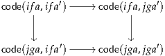 | (8.7.2) |
This amounts to saying that if we add something to the beginning and then something to the end of a sequence, we might as well have done it in the other order.
Remark 8.7.3. One might expect to see in the definition of code some additional generating equations for the set-quotient, such as
| (…, pk-1 ▪fw, xk′, qk, …) | = (…, pk-1, xk, gw▪qk, …) | (for w : Π1 A(xk , xk ′)) |
| (…, qk ▪gw, yk′, pk, …) | = (…, qk, yk, fw▪pk, …). | (for w : Π1 A(yk , yk ′)) |
Continuing on, we can characterize transporting in the fibration code:


Here we are abusing notation by using the same name for a path in X and its image in Π1X. Note that transport in Π1X is also given by concatenation with (the image of) a path. From this we can prove the above statements by induction on u. We also have:

This follows essentially from the definition of code.
We also construct a function
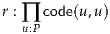
by induction on u as follows:
| rib | :≡ (b, reflb, b) | ||
| rjc | :≡ (c, reflc, c) |
| (ka, ka)*(fa, reflfa, fa) | = (ga, reflga, a, reflfa, a, reflga, ga) | ||
| = (ga, reflga, ga) |
We will now prove:
Proof.
To define a function

it suffices to define a function (u = Pv) →code(u, v), since code(u, v) is a set. We do this by transport:

Now to define

we proceed as usual by induction on u, v : P. In each case for u and v, we apply i or j to all the equalities pk and qk as appropriate and concatenate the results in P, using h to identify the endpoints. For instance, when u ≡ ib and v ≡ ib′, we define

As usual, to show that the composite

is the identity, we first peel off the 0-truncation (since the codomain is a set) and then apply path induction. The input reflu goes to ru, which then goes back to reflu (applying a further induction on u to decompose decode(ru)).
Finally, consider the composite

We proceed by induction on u, v : P. When u ≡ ib and v ≡ ib′, this composite is
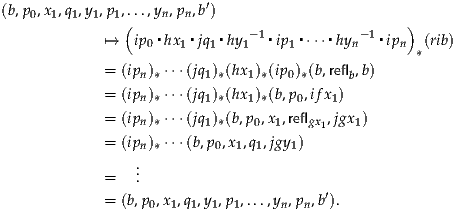
Theorem 8.7.4 allows us to calculate the fundamental groups of many types, provided A is a set, for in that case, each code(u, v) is, by definition, a set-quotient of a set by a relation.
Example 8.7.6. Let A :≡2, B :≡1, and C :≡1. Then P ≃ S1. Inspecting
the definition of, say, code(i(⋆), i(⋆)), we see that the paths all may as
well be trivial, so the only information is in the sequence of elements
x1, y1, …, xn, yn : 2. Moreover, if we have xk = yk or yk = xk+1 for any k,
then the set-quotient relations allow us to excise both of those elements.
Thus, every such sequence is equal to a canonical reduced one in which
no two adjacent elements are equal. Clearly such a reduced sequence is
uniquely determined by its length (a natural number n) together with, if
n > 1, the information of whether x1 is 02 or 12, since that determines the
rest of the sequence uniquely. And these data can, of course, be identified
with an integer, where n is the absolute value and x1 encodes the sign.
Thus we recover π1(S1) Z.
Z.
Since Theorem 8.7.4 asserts only a bijection of families of sets, this
isomorphism π1(S1) Z is likewise only a bijection of sets. We could,
however, define a concatenation operation on code (by concatenating
sequences) and show that encode and decode form an isomorphism respecting
this structure. (In the language of Chapter 9, these would be “pregroupoids”.)
We leave the details to the reader.
Z is likewise only a bijection of sets. We could,
however, define a concatenation operation on code (by concatenating
sequences) and show that encode and decode form an isomorphism respecting
this structure. (In the language of Chapter 9, these would be “pregroupoids”.)
We leave the details to the reader.
Example 8.7.7. More generally, let B :≡1 and C :≡1 but A be arbitrary, so that P is the suspension of A. Then once again the paths pk and qk are trivial, so that the only information in a path code is a sequence of elements x1, y1, …, xn, yn : A. The first two generating equalities say that adjacent equal elements can be canceled, so it makes sense to think of this sequence as a word of the form
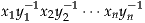
in a group. Indeed, it looks similar to the free group on A (or
equivalently on  0; see Remark 6.11.8), but we are considering
only words that start with a non-inverted element, alternate between
inverted and non-inverted elements, and end with an inverted one. This
effectively reduces the size of the generating set by one. For instance, if A
has a point a : A, then we can identify π1(ΣA) with the group presented
by
0; see Remark 6.11.8), but we are considering
only words that start with a non-inverted element, alternate between
inverted and non-inverted elements, and end with an inverted one. This
effectively reduces the size of the generating set by one. For instance, if A
has a point a : A, then we can identify π1(ΣA) with the group presented
by  0 as generators with the relation
  0 = e; see Exercises 8.10
and 8.11 for details.
0 = e; see Exercises 8.10
and 8.11 for details.
Example 8.7.8. Let A :≡ 1 and B and C be arbitrary, so that f and g
simply equip B and C with basepoints b and c, say. Then P is the wedge
B ∨C of B and C (the coproduct in the category of based spaces). In
this case, it is the elements xk and yk which are trivial, so that the only
information is a sequence of loops (p0, q1, p1, …, pn) with pk : π1(B, b)
and qk : π1(C, c). Such sequences, modulo the equivalence relation we
have imposed, are easily identified with the explicit description of the
free product of the groups π1(B, b) and π1(C, c), as constructed in §6.11.
Thus, we have π1(B∨C) π1(B) *π1(C).
However, Theorem 8.7.4 stops just short of being the full classical van
Kampen theorem, which handles the case where A is not necessarily a
set, and states that π1(B⊔AC) π1(B) *π1(A)π1(C) (with base point
coming from A). Indeed, the conclusion of Theorem 8.7.4 says nothing at
all about π1(A); the paths in A are “built into the quotienting” in a
type-theoretic way that makes it hard to extract explicit information, in that
code(u, v) is a set-quotient of a non-set by a relation. For this reason, in
the next subsection we consider a better version of the van Kampen
theorem.
π1(B) *π1(A)π1(C) (with base point
coming from A). Indeed, the conclusion of Theorem 8.7.4 says nothing at
all about π1(A); the paths in A are “built into the quotienting” in a
type-theoretic way that makes it hard to extract explicit information, in that
code(u, v) is a set-quotient of a non-set by a relation. For this reason, in
the next subsection we consider a better version of the van Kampen
theorem.
The improvement of van Kampen we present now is closely analogous to a similar improvement in classical algebraic topology, where A is equipped with a set Sof base points. In fact, it turns out to be unnecessary for our proof to assume that the “set of basepoints” is a set — it might just as well be an arbitrary type; the utility of assuming S is a set arises later, when applying the theorem to obtain computations. What is important is that S contains at least one point in each connected component of A. We state this in type theory by saying that we have a type S and a function k : S → A which is surjective, i.e. (-1)-connected. If S ≡ A and k is the identity function, then we will recover the naive van Kampen theorem. Another example to keep in mind is when A is pointed and (0-)connected, with k : 1 → A the point: by Lemmas 7.5.2 and 7.5.11 this map is surjective just when A is 0-connected.
Let A, B, C, f, g, P, i, j, h be as in the previous section. We now define, given our surjective map k : S → A, an auxiliary type which improves the connectedness of k. Let T be the higher inductive type generated by
There is an obvious induced function k : T → A such that k ℓ = k, and any
p : ks = ks′ is equal to the composite ks = k ℓs k ℓs′ = ks′.
Proof. We must show that for all a : A, the 0-truncation of the type
∑
(t:T) (k t = a) is contractible. Since contractibility is a mere proposition
and k is (-1)-connected, we may assume that a = ks for some s : S.
Now we can take the center of contraction to be  0 where q is the
equality k ℓs = ks.
0 where q is the
equality k ℓs = ks.
It remains to show that for any ϕ : 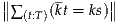 0 we have
ϕ =
0 we have
ϕ =  0. Since the latter is a mere proposition, and in particular a
set, we may assume that ϕ =
0. Since the latter is a mere proposition, and in particular a
set, we may assume that ϕ =  0 for t : T and p : k t = ks.
Now we can do induction on t : T. If t ≡ ℓs′, then ks′ = k ℓs′ ks
yields via m an equality ℓs = ℓs′. Hence by definition of k and of
equality in homotopy fibers, we obtain an equality (ks′, p) = (ks, q),
and thus
ks
yields via m an equality ℓs = ℓs′. Hence by definition of k and of
equality in homotopy fibers, we obtain an equality (ks′, p) = (ks, q),
and thus  0 =
0 =  0. Next we must show that as t varies
along m these equalities agree. But they are equalities in a set (namely
0. Next we must show that as t varies
along m these equalities agree. But they are equalities in a set (namely
 0), and hence this is automatic. __
Remark 8.7.10. T can be regarded as the (homotopy) coequalizer of the “kernel pair” of k. If S and A were sets, then the (-1)-connectivity of k would imply that A is the 0-truncation of this coequalizer (see Chapter 10). For general types, higher topos theory suggests that (-1)-connectivity of k will imply instead that A is the colimit (a.k.a. “geometric realization”) of the “simplicial kernel” of k. The type T is the colimit of the “1-skeleton” of this simplicial kernel, so it makes sense that it improves the connectivity of k by 1. More generally, we might expect the colimit of the n-skeleton to improve connectivity by n.
Now we define code : P → P → by double induction as follows

where
The quotient is generated by the following equalities (see Remark 8.7.3):
decode on such a sequence, which as before concatenates all the paths pk and qk together with instances of h to give an element of Π1P(ifb, ifb′), cf. (8.7.5). As before, the other three point cases are nearly identical.
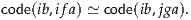 | (8.7.11) |
Since code is set-valued, by Lemma 8.7.9 we may assume that a = k t for some t : T. Next, we can do induction on t. If t ≡ ℓs for s : S, then we define (8.7.11) as in §8.7.1:
| (…, yn, pn, fks) |  (…, yn, pn, s, reflgks, gks), (…, yn, pn, s, reflgks, gks), | ||
| (…, xn, pn, s, reflfks, fks) | ← (…, xn, pn, gks). |

is mapped by (8.7.11) to

But this follows directly from the new generators we have imposed on the set-quotient relation defining code.
Theorem 8.7.12 (van Kampen with a set of basepoints). For all u, v : P there is an equivalence
with code defined as in this section.
Proof. Basically just like before. To show that decode respects the new generators of the quotient relation, we use the naturality of h. And to show that decode respects the equivalences such as (8.7.11), we need to induct on k and on T in order to decompose those equivalences into their definitions, but then it becomes again simply functoriality of f and g. The rest is easy. In particular, no additional argument is required for encode ∘decode, since the goal is to prove an equality in a set, and so the case of h is trivial. __
Theorem 8.7.12 allows us to calculate the fundamental group of a space A, even when A is not a set, provided S is a set, for in that case, each code(u, v) is, by definition, a set-quotient of a set by a relation. In that respect, it is an improvement over Theorem 8.7.4.
Example 8.7.13. Suppose S :≡1, so that A has a basepoint a :≡ k(⋆) and is connected. Then code for loops in the pushout can be identified with alternating sequences of loops in π1(B, f(a)) and π1(C, g(a)), modulo an equivalence relation which allows us to slide elements of π1(A, a) between them (after applying f and g respectively). Thus, π1(P) can be identified with the amalgamated free product π1(B) *π1(A)π1(C) (the pushout in the category of groups), as constructed in §6.11. This (in the case when B and C are open subspaces of P and A their intersection) is probably the most classical version of the van Kampen theorem.
Example 8.7.14. As a special case of Example 8.7.13, suppose additionally that C :≡1, so that P is the cofiber B/A. Then every loop in C is equal to reflexivity, so the relations on path codes allow us to collapse all sequences to a single loop in B. The additional relations require that multiplying on the left, right, or in the middle by an element in the image of π1(A) is the identity. We can thus identify π1(B/A) with the quotient of the group π1(B) by the normal subgroup generated by the image of π1(A).
Example 8.7.15. As a further special case of Example 8.7.14, let B :≡ S1 ∨S1, let A :≡ S1, and let f : A → B pick out the composite loop p▪q▪p-1 ▪q-1, where p and q are the generating loops in the two copies of S1 comprising B. Then P is a presentation of the torus T2. Indeed, it is not hard to identify P with the presentation of T2 as described in §6.7, using the cone on a particular loop. Thus, π1(T2) is the quotient of the free group on two generators (i.e., π1(B)) by the relation p▪q▪p-1 ▪q-1 = 1. This clearly yields the free abelian group on two generators, which is Z ×Z.
Example 8.7.16. More generally, any CW complex can be obtained by repeatedly “coning off” spheres, as described in §6.7. That is, we start with a set X0 of points (“0-cells”), which is the “0-skeleton” of the CW complex. We take the pushout
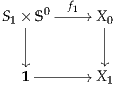 |
for some set S1 of 1-cells and some family f1 of “attaching maps”, obtaining the “1-skeleton” X1. Then we take the pushout
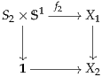 |
for some set S2 of 2-cells and some family f2 of attaching maps, obtaining the 2-skeleton X2, and so on. The fundamental group of each pushout can be calculated from the van Kampen theorem: we obtain the group presented by generators derived from the 1-skeleton, and relations derived from S2 and f2. The pushouts after this stage do not alter the fundamental group, since π1(Sn) is trivial for n > 1 (see §8.3).
Example 8.7.17. In particular, suppose given any presentation of a
(set-)group G = ⟨X∣R⟩, with X a set of generators and R a set of words
in these generators. Let B :≡ ∨
XS1 and A :≡ ∨RS1, with f : A → B
sending each copy of S1 to the corresponding word in the generating
loops of B. It follows that π1(P) G; thus we have constructed a
connected type whose fundamental group is G. Since any group has a
presentation, any group is the fundamental group of some type. If we
1-truncate such a type, we obtain a type whose only nontrivial homotopy
group is G; this is called an Eilenberg–Mac Lane space K(G, 1).
G; thus we have constructed a
connected type whose fundamental group is G. Since any group has a
presentation, any group is the fundamental group of some type. If we
1-truncate such a type, we obtain a type whose only nontrivial homotopy
group is G; this is called an Eilenberg–Mac Lane space K(G, 1).
In classical homotopy theory, a map f : A → B which induces an isomorphism
πn(A, a) πn(B, f(a)) for all points a in A (and also an isomorphism
π0(A)
πn(B, f(a)) for all points a in A (and also an isomorphism
π0(A) π0(B)) is necessarily a homotopy equivalence, as long as the spaces
A and B are well-behaved (e.g. have the homotopy types of CW-complexes).
This is known as Whitehead’s theorem. In fact, the “ill-behaved” spaces for
which Whitehead’s theorem fails are invisible to type theory. Roughly, the
well-behaved topological spaces suffice to present ∞-groupoids, and
homotopy type theory deals with ∞-groupoids directly rather than actual
topological spaces. Thus, one might expect that Whitehead’s theorem would
be true in univalent foundations.
π0(B)) is necessarily a homotopy equivalence, as long as the spaces
A and B are well-behaved (e.g. have the homotopy types of CW-complexes).
This is known as Whitehead’s theorem. In fact, the “ill-behaved” spaces for
which Whitehead’s theorem fails are invisible to type theory. Roughly, the
well-behaved topological spaces suffice to present ∞-groupoids, and
homotopy type theory deals with ∞-groupoids directly rather than actual
topological spaces. Thus, one might expect that Whitehead’s theorem would
be true in univalent foundations.
However, this is not the case: Whitehead’s theorem is not provable. In fact, there are known models of type theory in which it fails to be true, although for entirely different reasons than its failure for ill-behaved topological spaces. These models are “non-hypercomplete ∞-toposes” (see [Lur09]); roughly speaking, they consist of sheaves of ∞-groupoids over ∞-dimensional base spaces.
From a foundational point of view, therefore, we may speak of Whitehead’s principle as a “classicality axiom”, akin to LEM and AC. It may consistently be assumed, but it is not part of the computationally motivated type theory, nor does it hold in all natural models. But when working from set-theoretic foundations, this principle is invisible: it cannot fail to be true in a world where ∞-groupoids are built up out of sets (using topological spaces, simplicial sets, or any other such model).
This may seem odd, but actually it should not be surprising. Homotopy type theory is the abstract theory of homotopy types, whereas the homotopy theory of topological spaces or simplicial sets in set theory is a concrete model of this theory, in the same way that the integers are a concrete model of the abstract theory of rings. It is to be expected that any concrete model will have special properties which are not intrinsic to the corresponding abstract theory, but which we might sometimes want to assume as additional axioms (e.g. the integers are a Principal Ideal Domain, but not all rings are).
It is beyond the scope of this book to describe any models of type theory, so we will not explain how Whitehead’s principle might fail in some of them. However, we can prove that it holds whenever the types involved are n-truncated for some finite n, by “downward” induction on n. In addition to being of interest in its own right (for instance, it implies the essential uniqueness of Eilenberg–Mac Lane spaces), the proof of this result will hopefully provide some intuitive explanation for why we cannot hope to prove an analogous theorem without truncation hypotheses.
We begin with the following modification of Theorem 4.6.3, which will eventually supply the induction step in the proof of the truncated Whitehead’s principle. It may be regarded as a type-theoretic, ∞-groupoidal version of the classical statement that a fully faithful and essentially surjective functor is an equivalence of categories.
Theorem 8.8.1. Suppose f : A → B is a function such that
 0 :
0 :  0 →
0 → 0 is surjective, and
Then f is an equivalence.
Proof. Note that (ii) is precisely the statement that f is an embedding,
c.f. §4.6. Thus, by Theorem 4.6.3, it suffices to show that f is surjective,
i.e. that for any b : B we have  -1. Suppose given b; then since
 0 is surjective, there merely exists an a : A such that
  0(
0( 0) =
0) =
 0. And since our goal is a mere proposition, we may assume given
such an a. Then we have
0. And since our goal is a mere proposition, we may assume given
such an a. Then we have  0 =
0 =  0(
0( 0) =
0) =  0, hence
 -1. Again, since our goal is still a mere proposition, we
may assume f(a) = b. Hence fibf(b) is inhabited, and thus merely
inhabited. __
-1. Again, since our goal is still a mere proposition, we
may assume f(a) = b. Hence fibf(b) is inhabited, and thus merely
inhabited. __
Since homotopy groups are truncations of loop spaces, rather than path spaces, we need to modify this theorem to speak about these instead.
Corollary 8.8.2. Suppose f : A → B is a function such that
 0 :
0 :  0 →
0 → 0 is a bijection, and
Then f is an equivalence.
Proof. By Theorem 8.8.1, it suffices to show that apf : (x =A y) → (f(x) =B f(y))
is an equivalence for any x, y : A. And by Corollary 4.4.6, we may
assume f(x) =B f(y). In particular,  0 =
0 =  0, so since
  0 is
an equivalence, we have
0 is
an equivalence, we have  0 =
0 =  0, hence
  -1. Since we are
trying to prove a mere proposition (f being an equivalence), we may
assume given p : x = y. But now the following square commutes up to
homotopy:
-1. Since we are
trying to prove a mere proposition (f being an equivalence), we may
assume given p : x = y. But now the following square commutes up to
homotopy:
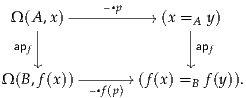 |
The top and bottom maps are equivalences, and the left-hand map is so by assumption. Hence, by the 2-out-of-3 property, so is the right-hand map. __
Now we can prove the truncated Whitehead’s principle.
Theorem 8.8.3. Suppose A and B are n-types and f : A → B is such that
 0 :
0 :  0 →
0 → 0 is an isomorphism, and
Then f is an equivalence.
Condition (i) is almost the case of (ii) when k = 0, except that it makes no reference to any basepoint x : A.
Proof. We proceed by induction on n. When n = -2, the statement is trivial. Thus, suppose it to be true for all functions between n-types, and let A and B be (n + 1)-types and f : A → B as above. The first condition in Corollary 8.8.2 holds by assumption, so it will suffice to show that for any x : A, the function apf : Ω(A, x) → Ω(B, f(x)) is an equivalence. However, Ω(A, x) and Ω(B, f(x)) are n-types, and πk(apf) = πk+1(f), so this follows from the inductive hypothesis. __
Note that if A and B are not n-types for any finite n, then there is no way for the induction to get started.
Corollary 8.8.4. If A is a 0-connected n-type and πk(A, a) = 0 for all k and a : A, then Ais contractible.
Proof. Apply Theorem 8.8.3 to the map A →1. __
As an application, we can deduce the converse of Corollary 8.4.8.
Corollary 8.8.5. For n ≥ 0, a map f : A → B is n-connected if and only if the following all hold:
 0 :
0 :  0 →
0 → 0 is an isomorphism.
Proof. The “only if” direction is Corollary 8.4.8. Conversely, by the long
exact sequence of a fibration (Theorem 8.4.6), the hypotheses imply that
πk(fibf(f(a))) = 0 for all k ≤ n and a : A, and that  0 is
contractible. Since πk(fibf(f(a))) = πk(
0 is
contractible. Since πk(fibf(f(a))) = πk( n) for k ≤ n, and
 n is n-connected, by Corollary 8.8.4 it is contractible for any
a.
n is n-connected, by Corollary 8.8.4 it is contractible for any
a.
It remains to show that  n is contractible for b : B not
necessarily of the form f(a). However, by assumption, there is x :
n is contractible for b : B not
necessarily of the form f(a). However, by assumption, there is x :  0
with
0
with  0 =
0 =  0(x). Since contractibility is a mere proposition, we may
assume x is of the form
0(x). Since contractibility is a mere proposition, we may
assume x is of the form  0 for a : A, in which case
  0 =
0 =  0(
0( 0) =
0) =
 0, and therefore
  -1. Again since contractibility is a
mere proposition, we may assume b = f(a), and the result follows. __
-1. Again since contractibility is a
mere proposition, we may assume b = f(a), and the result follows. __
A map f such that  0 is a bijection and πk(f) is a bijection for all k is
called ∞-connected or a weak equivalence. This is equivalent to asking that f
be n-connected for all n. A type Z is called ∞-truncated or hypercomplete if
the induced map
0 is a bijection and πk(f) is a bijection for all k is
called ∞-connected or a weak equivalence. This is equivalent to asking that f
be n-connected for all n. A type Z is called ∞-truncated or hypercomplete if
the induced map

is an equivalence whenever f is ∞-connected — that is, if Z thinks every ∞-connected map is an equivalence. Then if we want to assume Whitehead’s principle as an axiom, we may use either of the following equivalent forms.
In higher topos models, the ∞-truncated types form a reflective subuniverse in the sense of §7.7 (the “hypercompletion” of an (∞, 1)-topos), but we do not know whether this is true in general.
It may not be obvious that there are any types which are not n-types for any n, but in fact there are. Indeed, in classical homotopy theory, Sn has this property for any n ≥ 2. We have not proven this fact in homotopy type theory yet, but there are other types which we can prove to have “infinite truncation level”.
Example 8.8.6. Suppose we have B : N → such that for each n, the type
B(n) contains an n-loop which is not equal to n-fold reflexivity, say pn :
Ωn(B(n), bn) with pn≠reflbnn. (For instance, we could define B(n) :≡Sn,
with pn the image of 1 : Z under the isomorphism πn(Sn) Z.) Consider
C :≡ ∏(n:N) B(n), with the point c : C defined by c(n) :≡ bn. Since loop
spaces commute with products, for any m we have
Z.) Consider
C :≡ ∏(n:N) B(n), with the point c : C defined by c(n) :≡ bn. Since loop
spaces commute with products, for any m we have
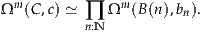
Under this equivalence, reflcm corresponds to the function (n reflbnm).
Now define qm in the right-hand type by
reflbnm).
Now define qm in the right-hand type by
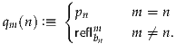
If we had qm = (n reflbnm), then we would have pn = reflbnn, which is
not the case. Thus, qm≠(n
reflbnm), then we would have pn = reflbnn, which is
not the case. Thus, qm≠(n reflbnm), and so there is a point of Ωm(C, c)
which is unequal to reflcm. Hence C is not an m-type, for any m : N.
reflbnm), and so there is a point of Ωm(C, c)
which is unequal to reflcm. Hence C is not an m-type, for any m : N.
We expect it should also be possible to show that a universe
itself is not an n-type for any n, using the fact that it contains higher
inductive types such as Sn for all n. However, this has not yet been
done.
We have used the encode-decode method to characterize the path spaces of various types, including coproducts (Theorem 2.12.5), natural numbers (Theorem 2.13.1), truncations (Theorem 7.3.12), the circle (Corollary 8.1.10), suspensions (Theorem 8.6.4), and pushouts (Theorem 8.7.12). Variants of this technique are used in the proofs of many of the other theorems mentioned in the introduction to this chapter, such as a direct proof of πn(Sn), the Blakers–Massey theorem, and the construction of Eilenberg–Mac Lane spaces. While it is tempting to try to abstract the method into a lemma, this is difficult because slightly different variants are needed for different problems. For example, different variations on the same method can be used to characterize a loop space (as in Theorem 2.12.5 and Corollary 8.1.10) or a whole path space (as in Theorem 2.13.1), to give a complete characterization of a loop space (e.g. Ω1(S1)) or only to characterize some truncation of it (e.g. van Kampen), and to calculate homotopy groups or to prove that a map is n-connected (e.g. Freudenthal and Blakers–Massey).
However, we can state lemmas for specific variants of the method. The proofs of these lemmas are almost trivial; the main point is to clarify the method by stating them in generality. The simplest case is using an encode-decode method to characterize the loop space of a type, as in Theorem 2.12.5 and Corollary 8.1.10.
Lemma 8.9.1 (Encode-decode for Loop Spaces). Given a pointed type (A, a0)
and a fibration code : A →, if
then (a0 = a0) is equivalent to code(a0).
Proof. Define encode : ∏(x:A) (a0 = x) →code(x) by

We show that encodea0 and decodea0 are quasi-inverses. The composition encodea0 ∘decodea0 is immediate by assumption (iii). For the other composition, we show
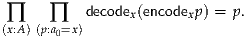
By path induction, it suffices to show decodea0(encodeaorefl) = refl. After reducing the transport, it suffices to show decodea0(c0) = refl, which is assumption (iv). __
If a fiberwise equivalence between (a0 = –) and code is desired, it suffices to strengthen condition (iii) to
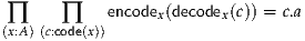
However, to calculate a loop space (e.g. Ω(S1)), this stronger assumption is not necessary.
Another variation, which comes up often when calculating homotopy groups, characterizes the truncation of a loop space:
Lemma 8.9.2 (Encode-decode for Truncations of Loop Spaces).
Assume a pointed type (A, a0) and a fibration code : A →, where for every
x, code(x) is a k-type. Define
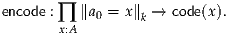
by truncation recursion (using the fact that code(x) is a k-type), mapping α : a0 = x to transportcode(α, c0). Suppose:
 k,
k,
 .
.Then  k is equivalent to code(a0).
Proof. That decode ∘encode is identity is immediate by (iii). To prove encode ∘decode, we first do a truncation induction, by which it suffices to show
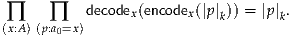
The truncation induction is allowed because paths in a k-type are a k-type. To show this type, we do a path induction, and after reducing the encode, use assumption (iv). __
Though we do not present the proofs in this chapter, following results have also been established in homotopy type theory.
Notes on the proof. The proof consists of a calculation of π4(S3), together with an appeal to stability (Corollary 8.6.15). In the classical statement of this result, k is 2. While we have not yet checked that k is in fact 2, our calcluation of π4(S3) is constructive, like all the rest of the proofs in this chapter. (More precisely, it doesn’t use any additional axioms such as LEM or AC, making it as constructive as univalence and higher inductive types are.) Thus, given a computational interpretation of homotopy type theory, we could run the proof on a computer to verify that k is 2. This example is quite intriguing, because it is the first calculation of a homotopy group for which we have not needed to know the answer in advance. __
Theorem 8.10.2 (Blakers–Massey theorem). Suppose we are given maps f : C → X, and g : C → Y. Taking first the pushout X⊔CY of f and g and then the pullback of its inclusions inl : X → X⊔CY ← Y : inr, we have an induced map C → X×(X⊔CY)Y.
If f is i-connected and g is j-connected, then this induced map is (i + j)-connected. In other words, for any points x : X, y : Y, the corresponding fiber Cx,y of (f, g) : C → X ×Y gives an approximation to the path space inl(x) =X⊔CY inr(y) in the pushout.
It should be noted that in classical algebraic topology, the Blakers–Massey theorem is often stated in a somewhat different form, where the maps f and g are replaced by inclusions of subcomplexes of CW complexes, and the homotopy pushout and homotopy pullback by a union and intersection, respectively. In order to express the theorem in homotopy type theory, we have to replace notions of this sort with ones that are homotopy-invariant. We have seen another example of this in the van Kampen theorem (§8.7), where we had to replace a union of open subsets by a homotopy pushout.
Theorem 8.10.3 (Eilenberg–Mac Lane Spaces). For any abelian group G and positive integer n, there is an n-type K(G, n) such that πn(K(G, n)) = G, and πk(K(G, n)) = 0 for k≠n.
Theorem 8.10.4 (Covering spaces). For a connected space A, there is an equivalence between covering spaces over Aand sets with an action of π1(A).
| Theorem | Status |
| π1(S1) | ✔✔ |
| πk<n(Sn) | ✔✔ |
| long-exact-sequence of homotopy groups | ✔✔ |
| total space of Hopf fibration is S3 | ✔ |
| π2(S2) | ✔✔ |
| π3(S2) | ✔ |
| πn(Sn) | ✔✔ |
| π4(S3) | ✔ |
| Freudenthal suspension theorem | ✔✔ |
| Blakers–Massey theorem | ✔✔ |
| Eilenberg–Mac Lane spaces K(G, n) | ✔✔ |
| van Kampen theorem | ✔✔ |
| covering spaces | ✔✔ |
| Whitehead’s principle for n-types | ✔✔ |
The theorems described in this chapter are standard results in classical homotopy theory; many are described by [Hat02]. In these notes, we review the development of the new synthetic proofs of them in homotopy type theory. Table 8.2 lists the homotopy-theoretic theorems that have been proven in homotopy type theory, and whether they have been computer-checked. Almost all of these results were developed during the spring term at IAS in 2013, as part of a significant collaborative effort. Many people contributed to these results, for example by being the principal author of a proof, by suggesting problems to work on, by participating in many discussions and seminars about these problems, or by giving feedback on results. The following people were the principal authors of the first homotopy type theory proofs of the above theorems. Unless indicated otherwise, for the theorems that have been computer-checked, the principal authors were also the first ones to formalize the proof using a computer proof assistant.
The interplay between homotopy theory and type theory was crucial to the development of these results. For example, the first proof that π1(S1) = Z was the one given in §8.1.5, which follows a classical homotopy theoretic one. A type-theoretic analysis of this proof resulted in the development of the encode-decode method. The first calculation of π2(S2) also followed classical methods, but this led quickly to an encode-decode proof of the result. The encode-decode calculation generalized to πn(Sn), which in turn led to the proof of the Freudenthal suspension theorem, by combining an encode-decode argument with classical homotopy-theoretic reasoning about connectedness, which in turn led to the Blakers–Massey theorem and Eilenberg–Mac Lane spaces. The rapid development of this series of results illustrates the promise of our new understanding of the connections between these two subjects.
Exercise 8.2. Prove that if A is a set with decidable equality (see Definition 3.4.3), then its suspension ΣA is a 1-type. (It is an open question whether this is provable without the assumption of decidable equality.)
Exercise 8.3. Define S∞ to be the colimit of the sequence S0 → S1 →
S2 → . Prove that S∞ is contractible.
Exercise 8.4. Define S∞ to be the higher inductive type generated by
In other words, S∞ is its own suspension. Prove that S∞ is contractible.
Exercise 8.5. Suppose f : X → Y is a function and Y is connected. Show
that for any y1, y2 : Y we have  .
.
Exercise 8.6. For any pointed type A, let iA : ΩA → ΩA denote inversion of loops, iA :≡ λp.p-1. Show that iΩA : Ω2A → Ω2A is equal to Ω(iA).
Exercise 8.7. Define a pointed equivalence to be a pointed map whose underlying function is an equivalence.
∙ (Y, y0).
Exercise 8.8. Following the example of the Hopf fibration in §8.5, define the junior Hopf fibration as a fibration (that is, a type family) over S1 whose fiber over the basepoint is S0 and whose total space is S1. This is also called the “twisted double cover” of the circle S1.
Exercise 8.9. Again following the example of the Hopf fibration in §8.5, define an analogous fibration over S4 whose fiber over the basepoint is S3 and whose total space is S7. This is an open problem in homotopy type theory (such a fibration is known to exist in classical homotopy theory).
Exercise 8.10. Continuing from Example 8.7.7, prove that if A has a
point a : A, then we can identify π1(ΣA) with the group presented by
 0 as generators with the relation
  0 = e. Then show that if we
assume excluded middle, this is also the free group on
0 = e. Then show that if we
assume excluded middle, this is also the free group on  0 \{
0 \{ 0}.
0}.
Exercise 8.11. Again continuing from Example 8.7.7, but this time without
assuming A to be pointed, show that we can identify π1(ΣA) with the group
presented by generators  0 ×
0 × 0 and relations
 |
Of the branches of mathematics, category theory is one which perhaps fits the least comfortably in set theoretic foundations. One problem is that most of category theory is invariant under weaker notions of “sameness” than equality, such as isomorphism in a category or equivalence of categories, in a way which set theory fails to capture. But this is the same sort of problem that the univalence axiom solves for types, by identifying equality with equivalence. Thus, in univalent foundations it makes sense to consider a notion of “category” in which equality of objects is identified with isomorphism in a similar way.
Ignoring size issues, in set-based mathematics a category consists of a set A0 of objects and, for each x, y ∈ A0, a set hom A(x, y) of morphisms. Under univalent foundations, a “naive” definition of category would simply mimic this with a type of objects and types of morphisms. If we allowed these types to contain arbitrary higher homotopy, then we ought to impose higher coherence conditions, leading to some notion of (∞, 1)-category, but at present our goal is more modest. We consider only 1-categories, and therefore we restrict the types hom A(x, y) to be sets, i.e. 0-types. If we impose no further conditions, we will call this notion a precategory.
If we add the requirement that the type A0 of objects is a set, then we end up with a definition that behaves much like the traditional set-theoretic one. Following Toby Bartels, we call this notion a strict category. But we can also require a generalized version of the univalence axiom, identifying (x = A0y) with the type iso(x, y) of isomorphisms from x to y. Since we regard this as usually the “correct” definition, we will call it simply a category.
A good example of the difference between the three notions of category is provided by the statement “every fully faithful and essentially surjective functor is an equivalence of categories”, which in classical set-based category theory is equivalent to the axiom of choice.
We will prove the latter statement in this chapter, as well as other pleasant
properties of categories, e.g. that equivalent categories are equal (as elements
of the type of categories). We will also describe a universal way of
“saturating” a precategory A into a category  , which we call its Rezk
completion, although it could also reasonably be called the stack completion (see
the Notes).
, which we call its Rezk
completion, although it could also reasonably be called the stack completion (see
the Notes).
The Rezk completion also sheds further light on the notion of equivalence
of categories. For instance, the functor A → is always fully faithful and
essentially surjective, hence a “weak equivalence”. It follows that a
precategory is a category exactly when it “sees” all fully faithful and
essentially surjective functors as equivalences; thus our notion of “category”
is already inherent in the notion of “fully faithful and essentially surjective
functor”.
is always fully faithful and
essentially surjective, hence a “weak equivalence”. It follows that a
precategory is a category exactly when it “sees” all fully faithful and
essentially surjective functors as equivalences; thus our notion of “category”
is already inherent in the notion of “fully faithful and essentially surjective
functor”.
We assume the reader has some basic familiarity with classical category
theory. Recall that whenever we write it denotes some universe of types,
but perhaps a different one at different times; everything we say remains true
for any consistent choice of universe levels. We will use the basic notions of
homotopy type theory from Chapters 1 and 2 and the propositional
truncation from Chapter 3, but not much else from Part I, except that our
second construction of the Rezk completion will use a higher inductive
type.
In classical mathematics, there are many equivalent definitions of a category. In our case, since we have dependent types, it is natural to choose the arrows to be a type family indexed by the objects. This matches the way hom-types are always used in category theory: we never even consider comparing two arrows unless we know their domains and codomains agree. Furthermore, it seems clear that for a theory of 1-categories, the hom-types should all be sets. This leads us to the following definition.
Definition 9.1.1. A precategory A consists of the following.

denoted infix by g f
f g∘f, or sometimes simply by gf.
 |
we have h∘ (g∘f) = (h∘g) ∘f.
The problem with the notion of precategory is that for objects a, b : A, we have two possibly-different notions of “sameness”. On the one hand, we have the type (a =A0 b). But on the other hand, there is the standard categorical notion of isomorphism.
Definition 9.1.2. A morphism f : hom A(a, b) is an isomorphism if
there is a morphism g : hom A(b, a) such that g∘f = 1a and f ∘g = 1b.
We write a b for the type of such isomorphisms.
Lemma 9.1.3. For any f : hom A(a, b), the type “f is an isomorphism” is a
mere proposition. Therefore, for any a, b : Athe type a b is a set.
Proof. Suppose given g : hom A(b, a) and η : (1a = g∘f) and ϵ : (f ∘g = 1b), and similarly g′, η′, and ϵ′. We must show (g, η, ϵ) = (g′, η′, ϵ′). But since all hom-sets are sets, their identity types are mere propositions, so it suffices to show g = g′. For this we have

using η and ϵ′. __
If f : a b, then we write f-1 for its inverse, which by Lemma 9.1.3 is
uniquely determined.
b, then we write f-1 for its inverse, which by Lemma 9.1.3 is
uniquely determined.
The only relationship between these two notions of sameness that we have in a precategory is the following.
Proof. By induction on identity, we may assume a and b are the same. But then we have 1a : hom A(a, a), which is clearly an isomorphism. __
Evidently, this situation is analogous to the issue that motivated us to introduce the univalence axiom. In fact, we have the following:
Example 9.1.5. There is a precategory et, whose type of objects is Set,
and with hom  et(A, B) :≡ (A → B). The identity morphisms are
identity functions and the composition is function composition. For this
precategory, Lemma 9.1.4 is equal to (the restriction to sets of) the map
idtoeqv from §2.10.
et(A, B) :≡ (A → B). The identity morphisms are
identity functions and the composition is function composition. For this
precategory, Lemma 9.1.4 is equal to (the restriction to sets of) the map
idtoeqv from §2.10.
Of course, to be more precise we should call this category et, since
its objects are only the small sets relative to a universe .
Thus, it is natural to make the following definition.
Definition 9.1.6. A category is a precategory such that for all a, b : A, the function idtoisoa,b from Lemma 9.1.4 is an equivalence.
In particular, in a category, if a b, then a = b.
Example 9.1.7. The univalence axiom implies immediately that et is a
category. One can also show, using univalence, that any precategory of
set-level structures such as groups, rings, topological spaces, etc. is a
category; see §9.8.
We also note the following.
Proof. It suffices to show that for any a, b : A, the type a = b is a set. But
a = b is equivalent to a b, which is a set. __
We write isotoid for the inverse (a b) → (a = b) of the map idtoiso
from Lemma 9.1.4. The following relationship between the two is
important.
b) → (a = b) of the map idtoiso
from Lemma 9.1.4. The following relationship between the two is
important.
Proof. By induction, we may assume p and q are refla and reflb respectively. Then the left-hand side of (9.1.10) is simply f. But by definition, idtoiso(refla) is 1a, and idtoiso(reflb) is 1b, so the right-hand side of (9.1.10) is 1b ∘f ∘ 1a, which is equal to f. __
Similarly, we can show
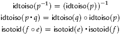 | (9.1.11) (9.1.12) (9.1.13) |
Example 9.1.14. A precategory in which each set hom A(a, b) is a mere proposition is equivalently a type A0 equipped with a mere relation “≤” that is reflexive (a ≤ a) and transitive (if a ≤ b and b ≤ c, then a ≤ c). We call this a preorder.
In a preorder, a witness f : a ≤ b is an isomorphism just when there
exists some witness g : b ≤ a. Thus, a b is the mere proposition that
a ≤ b and b ≤ a. Therefore, a preorder A is a category just when (1) each
type a = b is a mere proposition, and (2) for any a, b : A0 there exists
a function (a
b is the mere proposition that
a ≤ b and b ≤ a. Therefore, a preorder A is a category just when (1) each
type a = b is a mere proposition, and (2) for any a, b : A0 there exists
a function (a b) → (a = b). In other words, A0 must be a set, and ≤
must be antisymmetric (if a ≤ b and b ≤ a, then a = b). We call this a
(partial) order or a poset.
b) → (a = b). In other words, A0 must be a set, and ≤
must be antisymmetric (if a ≤ b and b ≤ a, then a = b). We call this a
(partial) order or a poset.
Example 9.1.15. If A is a category, then A0 is a set if and only if for any
a, b : A0, the type a b is a mere proposition. This is equivalent to saying
that every isomorphism in A is an identity; thus it is rather stronger
than the classical notion of “skeletal” category. Categories of this sort
are sometimes called gaunt [BSP11]. There is not really any notion of
“skeletality” for our categories, unless one considers Definition 9.1.6
itself to be such.
b is a mere proposition. This is equivalent to saying
that every isomorphism in A is an identity; thus it is rather stronger
than the classical notion of “skeletal” category. Categories of this sort
are sometimes called gaunt [BSP11]. There is not really any notion of
“skeletality” for our categories, unless one considers Definition 9.1.6
itself to be such.
Example 9.1.16. For any 1-type X, there is a category with X as its type of objects and with hom(x, y) :≡ (x = y). If X is a set, we call this the discrete category on X. In general, we call it a groupoid (see Exercise 9.6).
Example 9.1.17. For any type X, there is a precategory with X as its type
of objects and with hom(x, y) :≡ 0. The composition operation

is defined by induction on truncation from concatenation (y = z) → (x = y) → (x = z). We call this the fundamental pregroupoid of X. (In fact, we have met it already in §8.7; see also Exercise 9.11.)
Example 9.1.18. There is a precategory whose type of objects is and
with hom(X, Y) :≡  0, and composition defined by induction
on truncation from ordinary composition (Y → Z) → (X → Y) →
(X → Z). We call this the homotopy precategory of types.
0, and composition defined by induction
on truncation from ordinary composition (Y → Z) → (X → Y) →
(X → Z). We call this the homotopy precategory of types.
Example 9.1.19. Let  el be the following precategory:
 el(X, Y) = X → Y →Prop.
el(X, Y) and S : hom el(Y, Z), their composite is
defined by
el(X, Y) = X → Y →Prop.
el(X, Y) and S : hom el(Y, Z), their composite is
defined by
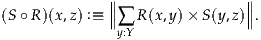
Suppose R : hom el(X, Y) is an isomorphism, with inverse S. We observe the
following.
In conclusion, if R : hom el(X, Y) is an isomorphism, then for each x : X there is
exactly one y : Y such that R(x, y), and dually. Thus, there is a function
f : X → Y sending each x to this y, which is an equivalence; hence X = Y.
With a little more work, we conclude that el is a category.
We might now restrict ourselves to considering categories rather than precategories. Instead, we will develop many concepts for precategories as well as categories, in order to emphasize how much better-behaved categories are, as compared both to precategories and to ordinary categories in classical mathematics.
We will also see in §§9.6–9.7 that in slightly more exotic contexts, there are uses for certain kinds of precategories other than categories, each of which “fixes” the equality of objects in different ways. This emphasizes the “pre”-ness of precategories: they are the raw material out of which multiple important categorical structures can be defined.
The following definitions are fairly obvious, and need no modification.
Definition 9.2.1. Let A and B be precategories. A functor F : A → B consists of
Note that by induction on identity, a functor also preserves idtoiso.
Definition 9.2.2. For functors F, G : A → B, a natural transformation γ : F → G consists of
Since each type hom B(Fa, Gb) is a set, its identity type is a mere proposition. Thus, the naturality axiom is a mere proposition, so identity of natural transformations is determined by identity of their components. In particular, for any F and G, the type of natural transformations from F to G is again a set.
Similarly, identity of functors is determined by identity of the functions A0 → B0 and (transported along this) of the corresponding functions on hom-sets.
Definition 9.2.3. For precategories A, B, there is a precategory BA defined by
Proof. We define (1F)a :≡ 1Fa. Naturality follows by the unit axioms of a precategory. For γ : F → G and δ : G → H, we define (δ∘γ)a :≡ δa∘γa. Naturality follows by associativity. Similarly, the unit and associativity laws for BA follow from those for B. __
Lemma 9.2.4. A natural transformation γ : F → G is an isomorphism in BA if and only if each γa is an isomorphism in B.
Proof. If γ is an isomorphism, then we have δ : G → F that is its inverse. By definition of composition in BA, (δγ)a ≡ δaγa and similarly. Thus, δγ = 1F and γδ = 1G imply δaγa = 1Fa and γaδa = 1Ga, so γa is an isomorphism.
Conversely, suppose each γa is an isomorphism, with inverse called δa, say. We define a natural transformation δ : G → F with components δa; for the naturality axiom we have

Now since composition and identity of natural transformations is determined on their components, we have γδ = 1G and δγ = 1F. __
The following result is fundamental.
Proof. Let F, G : A → B; we must show that idtoiso : (F = G) → (F G)
is an equivalence.
G)
is an equivalence.
To give an inverse to it, suppose γ : F G is a natural isomorphism.
Then for any a : A, we have an isomorphism γa : Fa
G is a natural isomorphism.
Then for any a : A, we have an isomorphism γa : Fa Ga, hence an
identity isotoid(γa) : Fa = Ga. By function extensionality, we have an
identity : F0 =(A0→B0) G0.
Ga, hence an
identity isotoid(γa) : Fa = Ga. By function extensionality, we have an
identity : F0 =(A0→B0) G0.
Now since the last two axioms of a functor are mere propositions, to show that F = G it will suffice to show that for any a, b : A, the functions
| Fa,b | : hom A(a, b) → hom B(Fa, Fb) | ||
| Ga,b | : hom A(a, b) → hom B(Ga, Gb) |
This completes the definition of a function (F G) → (F = G). Now
consider the composite
G) → (F = G). Now
consider the composite

Since hom-sets are sets, their identity types are mere propositions, so to show that two identities p, q : F = G are equal, it suffices to show that p =F0=G0 q. But in the definition of , if γ were of the form idtoiso(p), then γa would be equal to idtoiso(pa) (this can easily be proved by induction on p). Thus, isotoid(γa) would be equal to pa, and so by function extensionality we would have = p, which is what we need.
Finally, consider the composite

Since identity of natural transformations can be tested componentwise, it suffices to show that for each a we have idtoiso()a = γa. But as observed above, we have idtoiso()a = idtoiso(()a), while ()a = isotoid(γa) by computation for function extensionality. Since isotoid and idtoiso are inverses, we have idtoiso()a = γa as desired. __
In particular, naturally isomorphic functors between categories (as opposed to precategories) are equal.
We now define all the usual ways to compose functors and natural transformations.
Definition 9.2.6. For functors F : A → B and G : B → C, their composite G∘F : A → C is given by

It is easy to check the axioms.
Definition 9.2.7. For functors F : A → B and G, H : B → C and a natural transformation γ : G → H, the composite (γF) : GF → HF is given by
Naturality is easy to check. Similarly, for γ as above and K : C → D, the composite (Kγ) : KG → KH is given by
Lemma 9.2.8. For functors F, G : A → B and H, K : B → C and natural transformations γ : F → G and δ : H → K, we have
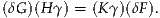
Proof. It suffices to check componentwise: at a : A we have
| ((δG)(Hγ))a | ≡ (δG)a(Hγ)a | ||
| ≡ δGa ∘H(γa) | |||
| = K(γa) ∘δFa | (by naturality of δ) | ||
| ≡ (Kγ)a ∘ (δF)a | |||
| ≡ ((Kγ)(δF))a. | __
Classically, one defines the “horizontal composite” of γ : F → G and δ : H → K to be the common value of (δG)(Hγ) and (Kγ)(δF). We will refrain from doing this, because while equal, these two transformations are not definitionally equal. This also has the consequence that we can use the symbol ∘ (or juxtaposition) for all kinds of composition unambiguously: there is only one way to compose two natural transformations (as opposed to composing a natural transformation with a functor on either side).
Proof. Since composition of functions is associative, this follows immediately for the actions on objects and on homs. And since hom-sets are sets, the rest of the data is automatic. __
The equality in Lemma 9.2.9 is likewise not definitional. (Composition of functions is definitionally associative, but the axioms that go into a functor must also be composed, and this breaks definitional associativity.) For this reason, we need also to know about coherence for associativity.
Proof. As in Lemma 9.2.9, this is evident for the actions on objects, and the rest is automatic. __
We will henceforth abuse notation by writing H∘G∘F or HGF for either H(GF) or (HG)F, transporting along Lemma 9.2.9 whenever necessary. We have a similar coherence result for units.
Lemma 9.2.11. For a functor F : A → B, we have equalities (1B ∘F) = F and (F ∘ 1A) = F, such that given also G : B → C, the following triangle of equalities commutes.
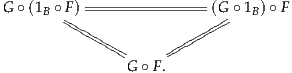
See Exercises 9.4 and 9.5 for further development of these ideas.
The definition of adjoint functors is straightforward; the main interesting aspect arises from proof-relevance.
The last two equations are called the triangle identities or zigzag identities. We leave it to the reader to define right adjoints analogously.
Lemma 9.3.2. If A is a category (but B may be only a precategory), then the type “F is a left adjoint” is a mere proposition.
Proof. Suppose we are given (G, η, ϵ) with the triangle identities and also (G′, η′, ϵ′). Define γ : G → G′ to be (G′ϵ)(η′G), and δ : G′→ G to be (Gϵ′)(ηG′). Then
| δγ | = (Gϵ′)(ηG′)(G′ϵ)(η′G) | ||
| = (Gϵ′)(GFG′ϵ)(ηG′FG)(η′G) | |||
| = (Gϵ)(Gϵ′FG)(GFη′G)(ηG) | |||
| = (Gϵ)(ηG) | |||
| = 1G |
 G′. By Theorem 9.2.5, we have an identity
G = G′.
G′. By Theorem 9.2.5, we have an identity
G = G′.
Now we need to know that when η and ϵ are transported along this identity, they become equal to η′ and ϵ′. By Lemma 9.1.9, this transport is given by composing with γ or δ as appropriate. For η, this yields
 |
using Lemma 9.2.8 and the triangle identity. The case of ϵ is similar. Finally, the triangle identities transport correctly automatically, since hom-sets are sets. __
In §9.5 we will give another proof of Lemma 9.3.2.
It is usual in category theory to define an equivalence of categories to be a
functor F : A → B such that there exists a functor G : B → A and natural
isomorphisms FG 1B and GF
 1A. Unlike the property of being an
adjunction, however, this would not be a mere proposition without truncating
it, for the same reasons that the type of quasi-inverses is ill-behaved (see §4.1).
And as in §4.2, we can avoid this by using the usual notion of adjoint
equivalence.
1A. Unlike the property of being an
adjunction, however, this would not be a mere proposition without truncating
it, for the same reasons that the type of quasi-inverses is ill-behaved (see §4.1).
And as in §4.2, we can avoid this by using the usual notion of adjoint
equivalence.
Definition 9.4.1. A functor F : A → B is an equivalence of (pre)categories if it is a left adjoint for which η and ϵ are isomorphisms. We write A ≃ B for the type of equivalences of categories from A to B.
By Lemmas 9.1.3 and 9.3.2, if A is a category, then the type “F is an equivalence of precategories” is a mere proposition.
Lemma 9.4.2. If for F : A → B there exists G : B → A and isomorphisms
GF 1A and FG
 1B, then F is an equivalence of precategories.
Proof. Just like the proof of Theorem 4.2.3 for equivalences of types. __
Definition 9.4.3. We say a functor F : A → B is faithful if for all a, b : A, the function

is injective, and full if for all a, b : A this function is surjective. If it is both (hence each Fa,b is an equivalence) we say F is fully faithful.
Definition 9.4.4. We say a functor F : A → B is split essentially
surjective if for all b : B there exists an a : A such that Fa b.
b.
Lemma 9.4.5. For any precategories Aand B and functor F : A → B, the following types are equivalent.
Proof. Suppose F is an equivalence of precategories, with G, η, ϵ specified. Then we have the function
| hom B(Fa, Fb) | → hom A(a, b), | ||
| g |  ηb-1 ∘G(g) ∘ηa. ηb-1 ∘G(g) ∘ηa. |

while for g : hom B(Fa, Fb) we have
| F(ηb-1 ∘G(g) ∘ηa) | = F(ηb-1) ∘F(G(g)) ∘F(ηa) | ||
| = ϵFb ∘F(G(g)) ∘F(ηa) | |||
| = g∘ϵFa ∘F(ηa) | |||
| = g |
 b.
b.
On the other hand, suppose F is fully faithful and split essentially
surjective. Define G0 : B0 → A0 by sending b : B to the a : A given by the
specified essential splitting, and write ϵb for the likewise specified
isomorphism FGb b.
b.
Now for any g : hom B(b, b′), define G(g) : hom A(Gb, Gb′) to be the unique morphism such that F(G(g)) = (ϵb′)-1 ∘g∘ϵ b (which exists since F is fully faithful). Finally, for a : A define ηa : hom A(a, GFa) to be the unique morphism such that Fηa = ϵFa-1. It is easy to verify that G is a functor and that (G, η, ϵ) exhibit F as an equivalence of precategories.
Now consider the composite (i)→(ii)→(i). We clearly recover the same function G0 : B0 → A0. For the action of G on hom-sets, we must show that for g : hom B(b, b′), G(g) is the (necessarily unique) morphism such that F(G(g)) = (ϵb′)-1 ∘g∘ϵ b. But this equation holds by the assumed naturality of ϵ. We also clearly recover ϵ, while η is uniquely characterized by Fηa = ϵFa-1 (which is one of the triangle identities assumed to hold in the structure of an equivalence of precategories). Thus, this composite is equal to the identity.
Finally, consider the other composite (ii)→(i)→(ii). Since being fully
faithful is a mere proposition, it suffices to observe that we recover, for each
b : B, the same a : A and isomorphism Fa b. But this is clear, since we used
this function and isomorphism to define G0 and ϵ in (i), which in turn are
precisely what we used to recover (ii) again. Thus, the composites in
both directions are equal to identities, hence we have an equivalence
(i) ≃(ii). __
b. But this is clear, since we used
this function and isomorphism to define G0 and ϵ in (i), which in turn are
precisely what we used to recover (ii) again. Thus, the composites in
both directions are equal to identities, hence we have an equivalence
(i) ≃(ii). __
However, if B is not a category, then neither type in Lemma 9.4.5 may necessarily be a mere proposition. This suggests considering as well the following notions.
Definition 9.4.6. A functor F : A → B is essentially surjective if for all
b : B, there merely exists an a : A such that Fa b. We say F is a weak
equivalence if it is fully faithful and essentially surjective.
b. We say F is a weak
equivalence if it is fully faithful and essentially surjective.
Being a weak equivalence is always a mere proposition. For categories, however, there is no difference between equivalences and weak ones.
Lemma 9.4.7. If F : A → B is fully faithful and Ais a category, then for any
b : B the type ∑(a:A) (Fa b) is a mere proposition. Hence a functor between
categories is an equivalence if and only if it is a weak equivalence.
b) is a mere proposition. Hence a functor between
categories is an equivalence if and only if it is a weak equivalence.
Proof. Suppose given (a, f) and (a′, f′) in ∑(a:A) (Fa b). Then f′-1 ∘f
is an isomorphism Fa
b). Then f′-1 ∘f
is an isomorphism Fa Fa′. Since F is fully faithful, we have g : a
 a′
with Fg = f′-1 ∘f. And since A is a category, we have p : a = a′
with idtoiso(p) = g. Now Fg = f′-1 ∘f implies ((F
0)
a′
with Fg = f′-1 ∘f. And since A is a category, we have p : a = a′
with idtoiso(p) = g. Now Fg = f′-1 ∘f implies ((F
0) )*
)* = f′,
hence (by the characterization of equalities in dependent pair types)
(a, f) = (a′, f′).
= f′,
hence (by the characterization of equalities in dependent pair types)
(a, f) = (a′, f′).
Thus, for fully faithful functors whose domain is a category, essential surjectivity is equivalent to split essential surjectivity, and so being a weak equivalence is equivalent to being an equivalence. __
This is an important advantage of our category theory over set-based approaches. With a purely set-based definition of category, the statement “every fully faithful and essentially surjective functor is an equivalence of categories” is equivalent to the axiom of choice AC. Here we have it for free, as a category-theoretic version of the principle of unique choice (§3.9). (In fact, this property characterizes categories among precategories; see §9.9.)
On the other hand, the following characterization of equivalences of categories is perhaps even more useful.
Definition 9.4.8. A functor F : A → B is an isomorphism of (pre)categories if F is fully faithful and F0 : A0 → B0 is an equivalence of types.
This definition is an exception to our general rule (see §2.4) of only using the word “isomorphism” for sets and set-like objects. However, it does carry an appropriate connotation here, because for general precategories, isomorphism is stronger than equivalence.
Note that being an isomorphism of precategories is always a mere
property. Let A B denote the type of isomorphisms of (pre)categories from
A to B.
B denote the type of isomorphisms of (pre)categories from
A to B.
Note that if B0 is not a 1-type, then (9.4.10) may not be a mere proposition.
Proof. First note that since hom-sets are sets, equalities between equalities of functors are uniquely determined by their object-parts. Thus, by function extensionality, (9.4.10) is equivalent to
 | (9.4.11) |
for all a : A0. Note that this is precisely the triangle identity for G0, η0, and ϵ0 to be a proof that F0 is a half adjoint equivalence of types.
Now suppose (i). Let G0 : B0 → A0 be the inverse of F0, with η0 : idA0 = G0F0 and ϵ0 : F0G0 = idB0 satisfying the triangle identity, which is precisely (9.4.11). Now define Gb,b′ : hom B(b, b′) → hom A(G0b, G0b′) by

(using the assumption that F is fully faithful). Since idtoiso takes inverses to inverses and concatenation to composition, and F is a functor, it follows that G is a functor.
By definition, we have (GF)0 ≡ G0F0, which is equal to idA0 by η0. To obtain 1A = GF, we need to show that when transported along η0, the identity function of hom A(a, a′) becomes equal to the composite GFa,Fa′∘Fa,a′. In other words, for any f : hom A(a, a′) we must have
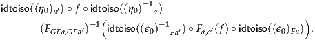 |
 |
On the other side, we have (FG)0 ≡ F0G0, which is equal to idB0 by ϵ0. To obtain FG = 1B, we need to show that when transported along ϵ0, the identity function of hom B(b, b′) becomes equal to the composite FGb,Gb′∘Gb,b′. That is, for any g : hom B(b, b′) we must have
 |
Conversely, suppose given (ii); then the object-parts of G, η, and ϵ together with (9.4.11) show that F0 is an equivalence of types. And for a, a′ : A0, we define Ga,a′ : hom B(Fa, Fa′) → hom A(a, a′) by
 | (9.4.12) |
By naturality of idtoiso(η), for any f : hom A(a, a′) we have
| Ga,a′(Fa,a′(f)) | = idtoiso(η-1)a ′∘G(F(f)) ∘idtoiso(η)a | ||
| = idtoiso(η-1)a ′∘idtoiso(η)a′∘f | |||
| = f. |
| Fa,a′(Ga,a′(g)) | = F(idtoiso(η-1)a ′) ∘F(G(g)) ∘F(idtoiso(η)a) | ||
| = idtoiso(ϵ)Fa′∘F(G(g)) ∘idtoiso(ϵ-1)Fa | |||
| = idtoiso(ϵ)Fa′∘idtoiso(ϵ-1)Fa ′∘g | |||
| = g. |
Now the composite (i)→(ii)→(i) is equal to the identity since (i) is a mere proposition. On the other side, tracing through the above constructions we see that the composite (ii)→(i)→(ii) essentially preserves the object-parts G0, η0, ϵ0, and the object-part of (9.4.10). And in the latter three cases, the object-part is all there is, since hom-sets are sets.
Thus, it suffices to show that we recover the action of G on hom-sets. In other words, we must show that if g : hom B(b, b′), then

where G is defined by (9.4.12). However, this follows from functoriality of G and the other triangle identity, which we have seen in Chapter 4 is equivalent to (9.4.11).
Now since (i) is a mere proposition, so is (ii), so it suffices to show they
are logically equivalent to (iii). Of course, (ii)→(iii), so let us assume (iii).
Since (i) is a mere proposition, we may assume given G, η, and ϵ. Then G0
along with η and ϵ imply that F0 is an equivalence. Moreover, we also have
natural isomorphisms idtoiso(η) : 1A GF and idtoiso(ϵ) : FG
 1B, so by
Lemma 9.4.2, F is an equivalence of precategories, and in particular fully
faithful. __
1B, so by
Lemma 9.4.2, F is an equivalence of precategories, and in particular fully
faithful. __
From Lemma 9.4.9(ii) and idtoiso in functor categories, we conclude immediately that any isomorphism of precategories is an equivalence. For precategories, the converse can fail.
Example 9.4.13. Let X be a type and x0 : X an element, and let Xch denote the chaotic or indiscrete precategory on X. By definition, we have (Xch)0 :≡ X, and hom Xch(x, x′) :≡ 1 for all x, x′. Then the unique functor Xch → 1 is an equivalence of precategories, but not an isomorphism unless X is contractible.
This example also shows that a precategory can be equivalent to a category without itself being a category. Of course, if a precategory is isomorphic to a category, then it must itself be a category.
However, for categories, the two notions coincide.
Lemma 9.4.14. For categories Aand B, a functor F : A → Bis an equivalence of categories if and only if it is an isomorphism of categories.
Proof. Since both are mere properties, it suffices to show they are logically equivalent. So first suppose F is an equivalence of categories, with (G, η, ϵ) given. We have already seen that F is fully faithful. By Theorem 9.2.5, the natural isomorphisms η and ϵ yield identities 1A = GF and FG = 1B, hence in particular identities idA = G0 ∘ F0 and F0 ∘G0 = idB. Thus, F0 is an equivalence of types.
Conversely, suppose F is fully faithful and F0 is an equivalence of
types, with inverse G0, say. Then for each b : B we have G0b : A
and an identity FGb = b, hence an isomorphism FGb b. Thus, by
Lemma 9.4.5, F is an equivalence of categories. __
b. Thus, by
Lemma 9.4.5, F is an equivalence of categories. __
Of course, there is yet a third notion of sameness for (pre)categories: equality. However, the univalence axiom implies that it coincides with isomorphism.
Lemma 9.4.15. If Aand B are precategories, then the function
(defined by induction from the identity functor) is an equivalence of types.
Proof. As usual for dependent sum types, to give an element of A = B is equivalent to giving

 = 1P0*
 and
and
 |
(Again, we use the fact that the identity types of hom-sets are mere propositions.) However, by univalence, this is equivalent to giving

But this consists exactly of a functor F : A → B that is an isomorphism of
categories. And by induction on identity, this equivalence (A = B) ≃ (A B)
is equal to the one obtained by induction. __
B)
is equal to the one obtained by induction. __
Thus, for categories, equality also coincides with equivalence. We can interpret this as saying that categories, functors, and natural transformations form, not just a pre-2-category, but a 2-category (see Exercise 9.4).
Theorem 9.4.16. If Aand B are categories, then the function
(defined by induction from the identity functor) is an equivalence of types.
As a consequence, the type of categories is a 2-type. For since A ≃ B is a subtype of the type of functors from A to B, which are the objects of a category, it is a 1-type; hence the identity types A = B are also 1-types.
Recall that we have a category et whose objects are sets and whose
morphisms are functions. We now show that every precategory has a
et-valued hom-functor. First we need to define opposites and products of
(pre)categories.
Definition 9.5.1. For a precategory A, its opposite Aop is a precategory with the same type of objects, with hom Aop (a, b) :≡ hom A(b, a), and with identities and composition inherited from A.
Definition 9.5.2. For precategories A and B, their product A×B is a precategory with (A×B)0 :≡ A0 ×B0 and

Identities are defined by 1(a,b) :≡ (1a, 1b) and composition by
 |
Lemma 9.5.3. For precategories A, B, C, the following types are equivalent.
Proof. Given F : A × B → C, for any a : A we obviously have a
functor Fa : B → C. This gives a function A0 → (CB)0. Next, for any
f : hom A(a, a′), we have for any b : B the morphism F(a,b),(a′,b)(f, 1b) :
Fa(b) → Fa′(b). These are the components of a natural transformation
Fa → Fa′. Functoriality in a is easy to check, so we have a functor
 : A → CB.
Conversely, suppose given G : A → CB. Then for any a : A and b : B we have the object G(a)(b) : C, giving a function A0 ×B0 → C0. And for f : hom A(a, a′) and g : hom B(b, b′), we have the morphism
 |
in hom C(G(a)(b), G(a′)(b′)). Functoriality is again easy to check, so we have a functor Ǧ : A×B → C.
Finally, it is also clear that these operations are inverses. __
Now for any precategory A, we have a hom-functor
It takes a pair (a, b) : (Aop)0 ×A0 ≡ A0 ×A0 to the set hom A(a, b). For a morphism (f, f′) : hom Aop×A((a, b), (a′, b′)), by definition we have f : hom A(a′, a) and f′ : hom A(b, b′), so we can define
| (hom A)(a,b),(a′,b′)(f, f′) | :≡ (g (f′gf)) (f′gf)) | ||
| : hom A(a, b) → hom A(a′, b′). |
By Lemma 9.5.3, therefore, we have an induced functor y : A →etAop
,
which we call the Yoneda embedding.
Theorem 9.5.4 (The Yoneda lemma). For any precategory A, any a : A, and any
functor F : etAop
, we have an isomorphism
 | (9.5.5) |
Moreover, this is natural in both aand F.
Proof. Given a natural transformation α : ya → F, we can consider
the component αa : ya(a) → Fa. Since ya(a) ≡ hom A(a, a), we have
1a : ya(a), so that αa(1a) : Fa. This gives a function (α αa(1a)) from left
to right in (9.5.5).
αa(1a)) from left
to right in (9.5.5).
In the other direction, given x : Fa, we define α : ya → F by
Naturality is easy to check, so this gives a function from right to left in (9.5.5).
To show that these are inverses, first suppose given x : Fa. Then with α defined as above, we have αa(1a) = Fa,a(1a)(x) = 1Fa(x) = x. On the other hand, if we suppose given α : ya → F and define x as above, then for any f : hom A(a′, a) we have
| αa′(f) | = αa′(yaa′,a(f)) | ||
| = (αa′∘yaa′,a(f))(1a) | |||
| = (Fa′,a(f) ∘αa)(1a) | |||
| = Fa′,a(f)(αa(1a)) | |||
| = Fa′,a(f)(x). |
Proof. By Theorem 9.5.4, we have

It is easy to check that this isomorphism is in fact the action of y on hom-sets. __
Corollary 9.5.7. If A is a category, then y0 : A0 → (etAop
)0 is an
embedding. In particular, if ya = yb, then a = b.
Proof. By Corollary 9.5.6, y induces an isomorphism on sets of
isomorphisms. But as A and etAop
are categories and y is a functor, this
is equivalently an isomorphism on identity types, which is the definition
of being an embedding. __
Definition 9.5.8. A functor F : etAop
is said to be representable if there
exists a : A and an isomorphism ya F.
F.
Proof. By definition “F is representable” is just the fiber of y0 over F. Since y0 is an embedding by Corollary 9.5.7, this fiber is a mere proposition. __
In particular, in a category, any two representations of the same functor are equal. We can use this to give a different proof of Lemma 9.3.2. First we give a characterization of adjunctions in terms of representability.
Lemma 9.5.10. For any precategories Aand B and a functor F : A → B, the following types are equivalent.
Proof. An element of the type (ii) consists of a function G0 : B0 → A0 together with, for every a : A and b : B an isomorphism

such that γa,b(g∘Ff) = γa′,b(g) ∘f for f : hom A(a, a′).
Given this, for a : A we define ηa :≡ γa,Fa(1Fa), and for b : B we define ϵb :≡ (γGb,b)-1(1 Gb). Now for g : hom B(b, b′) we define
The verifications that G is a functor and η and ϵ are natural transformations satisfying the triangle identities are exactly as in the classical case, and as they are all mere propositions we will not care about their values. Thus, we have a function (ii)→(i).
In the other direction, if F is a left adjoint, we of course have G0 specified, and we can take γa,b to be the composite

This is clearly natural since η is, and it has an inverse given by

(by the triangle identities). Thus we also have (i)→ (ii).
For the composite (ii)→(i)→ (ii), clearly the function G0 is preserved, so it suffices to check that we get back γ. But the new γ is defined to take f : hom B(Fa, b) to
| G(f) ∘ηa | ≡ γGFa,b(f ∘ϵFa) ∘ηa | ||
| = γGFa,b(f ∘ϵFa ∘Fηa) | |||
| = γGFa,b(f) |
Finally, for (i)→(ii)→ (i), we certainly get back the functor G on objects. The new Gb,b′ : hom B(b, b′) → hom A(Gb, Gb′) is defined to take g to
| γGb,b′(g∘ϵb) | ≡ G(g∘ϵb) ∘ηGb | ||
| = G(g) ∘Gϵb ∘ηGb | |||
| = G(g) |
Corollary 9.5.11. [Lemma 9.3.2] If A is a category and F : A → B, then the type “F is a left adjoint” is a mere proposition.
Proof. By Theorem 9.5.9, if A is a category then the type in Lemma 9.5.10(ii) is a mere proposition. __
In accordance with the mathematical red herring principle, a strict category is not necessarily a category. In fact, a category is a strict category precisely when it is gaunt (Example 9.1.15). Most of the time, category theory is about categories, not strict ones, but sometimes one wants to consider strict categories. The main advantage of this is that strict categories have a stricter notion of “sameness” than equivalence, namely isomorphism (or equivalently, by Lemma 9.4.15, equality).
Here is one origin of strict categories.
Example 9.6.2. Let A be a precategory and x : A an object. Then there is a precategory mono(A, x) as follows:
An equality (y, m) = (z, n) of objects in mono(A, x) consists of an equality
p : y = z and an equality p* = n, which by Lemma 9.1.9 is equivalently
an equality m = n∘idtoiso(p). Since hom-sets are sets, the type of such
equalities is a mere proposition. But since m and n are monomorphisms, the
type of morphisms f such that m = n∘f is also a mere proposition. Thus, if A
is a category, then (y, m) = (z, n) is a mere proposition, and hence mono(A, x)
is a strict category.
= n, which by Lemma 9.1.9 is equivalently
an equality m = n∘idtoiso(p). Since hom-sets are sets, the type of such
equalities is a mere proposition. But since m and n are monomorphisms, the
type of morphisms f such that m = n∘f is also a mere proposition. Thus, if A
is a category, then (y, m) = (z, n) is a mere proposition, and hence mono(A, x)
is a strict category.
This example can be dualized, and generalized in various ways. Here is an interesting application of strict categories.
Example 9.6.3. Let E/F be a finite Galois extension of fields, and G its Galois group. Then there is a strict category whose objects are intermediate fields F ⊆ K ⊆ E, and whose morphisms are field homomorphisms which fix F pointwise (but need not commute with the inclusions into E). There is another strict category whose objects are subgroups H ⊆ G, and whose morphisms are morphisms of G-sets G/H → G/K. The fundamental theorem of Galois theory says that these two precategories are isomorphic (not merely equivalent).
It is also worth mentioning a useful kind of precategory whose type of objects is not a set, but which is not a category either.
Definition 9.7.1. A †-precategory is a precategory A together with the following.
Definition 9.7.2. A morphism f : hom A(x, y) in a †-precategory is unitary if f†∘f = 1x and f ∘f† = 1y.
Of course, every unitary morphism is an isomorphism, and being unitary
is a mere proposition. Thus for each x, y : A we have a set of unitary
isomorphisms from x to y, which we denote (x  † y).
† y).
Proof. By induction, we may assume p is reflx. But then (1x)†∘ 1 x = 1x ∘ 1x = 1x and similarly. __
Definition 9.7.4. A †-category is a †-precategory such that for all x, y : A, the function
from Lemma 9.7.3 is an equivalence.
Example 9.7.5. The category el from Example 9.1.19 becomes a
†-precategory if we define (R†)(y, x) :≡ R(x, y). The proof that el is a
category actually shows that every isomorphism is unitary; hence el is
also a †-category.
Example 9.7.7. Let  ilb be the following precategory.
By standard linear algebra, any linear map f : V → W between finite
dimensional inner product spaces has a uniquely defined adjoint f† : W → V ,
characterized by ⟨fv, w⟩ = ⟨v, f†w⟩. In this way, ilb becomes a
†-precategory. Moreover, a linear isomorphism is unitary precisely when it is
an isometry, i.e. ⟨fv, fw⟩ = ⟨v, w⟩. It follows from this that ilb is a
†-category, though it is not a category (not every linear isomorphism is
unitary).
There has been a good deal of general theory developed for †-categories under classical foundations. It was observed early on that the unitary isomorphisms, not arbitrary isomorphisms, are the correct notion of “sameness” for objects of a †-category, which has caused some consternation among category theorists. Homotopy type theory resolves this issue by identifying †-categories, like strict categories, as simply a different kind of precategory.
The structure identity principle is an informal principle that expresses that isomorphic structures are identical. We aim to prove a general abstract result which can be applied to a wide family of notions of structure, where structures may be many-sorted or even dependently-sorted, infinitary, or even higher order.
The simplest kind of single-sorted structure consists of a type with no additional structure. The univalence axiom expresses the structure identity principle for that notion of structure in a strong form: for types A, B, the canonical function (A = B) → (A ≃ B) is an equivalence.
We start with a precategory X. In our application to single-sorted first
order structures, X will be the category of -small sets, where is a univalent
type universe.
Definition 9.8.1. A notion of structure (P, H) over X consists of the following.
. For each x : X0 the elements of Px are
called (P, H)-structures on x.

If Hαβ(f) is true, we say that f is a (P, H)-homomorphism from α to β.

When (P, H) is a notion of structure, for α, β : Px we define
By (iii) and (iv), this is a preorder (Example 9.1.14) with Px its type of objects. We say that (P, H) is a standard notion of structure if this preorder is in fact a partial order, for all x : X.
Note that for a standard notion of structure, each type Px must actually be a set. We now define, for any notion of structure (P, H), a precategory of (P, H)-structures, A = Str(P,H)(X).

The composition and identities are inherited from X; conditions (iii) and (iv) ensure that these lift to A.
Theorem 9.8.2 (Structure identity principle). If Xis a category and (P, H) is a standard notion of structure over X, then the precategory Str(P,H)(X) is a category.
Proof. By the definition of equality in dependent pair types, to give an equality (x, α) = (y, β) consists of
 = β.
= β.Since P is set-valued, the latter is a mere proposition. On the other hand, it is
easy to see that an isomorphism (x, α) (y, β) in Str(P,H)(X) consists
of
(y, β) in Str(P,H)(X) consists
of
 y in X, such that
Of course, the second of these is also a mere proposition. And since X is a
category, the function (x = y) → (x y) is an equivalence. Thus, it will suffice
to show that for any p : x = y and for any (α : Px), (β : Py), we have
p*
y) is an equivalence. Thus, it will suffice
to show that for any p : x = y and for any (α : Px), (β : Py), we have
p* = β if and only if both Hαβ(idtoiso(p)) and Hβα(idtoiso(p)-1).
The “only if” direction is just the existence of the function idtoiso for the category Str(P,H)(X). For the “if” direction, by induction on p we may assume that y ≡ x and p ≡reflx. However, in this case idtoiso(p) ≡ 1x and therefore idtoiso(p)-1 = 1 x. Thus, α ≤xβ and β ≤xα, which implies α = β since (P, H) is a standard notion of structure. __
As an example, this methodology gives an alternative way to express the proof of Theorem 9.2.5.
Example 9.8.3. Let A be a precategory and B a category. There is a
precategory BA0 whose objects are functions A0 → B0, and whose
set of morphisms from F0 : A0 → B0 to G0 : A0 → B0
is ∏(a:A0) hom B(F0a, G0a). Composition and identities are inherited
directly from those in B. It is easy to show that γ : hom BA0(F0, G0) is
an isomorphism exactly when each component γa is an isomorphism,
so that we have (F0 G0) ≃ ∏(a:A0) (F0a
 G0a). Moreover, the map
idtoiso : (F0 = G0) → (F0
G0a). Moreover, the map
idtoiso : (F0 = G0) → (F0 G0) of BA0 is equal to the composite

in which the first map is an equivalence by function extensionality, the second because it is a dependent product of equivalences (since B is a category), and the third as remarked above. Thus, BA0 is a category.
Now we define a notion of structure on BA0 for which P(F0) is the type of operations F : ∏(a,a′:A0) hom A(a, a′) → hom B(F0a, F0a′) which extend F0 to a functor (i.e. preserve composition and identities). This is a set since each hom B(–, –) is so. Given such F and G, we define γ : hom BA0(F0, G0) to be a homomorphism if it forms a natural transformation. In Definition 9.2.3 we essentially verified that this is a notion of structure. Moreover, if F and F′ are both structures on F0 and the identity is a natural transformation from F to F′, then for any f : hom A(a, a′) we have F′f = F′f ∘ 1F0a = 1F0a ∘Ff = Ff. Applying function extensionality, we conclude F = F′. Thus, we have a standard notion of structure, and so by Theorem 9.8.2, the precategory BA is a category.
As another example, we consider categories of structures for a first-order signature. We define a first-order signature, Ω, to consist of sets Ω0 and Ω1 of function symbols, ω : Ω0, and relation symbols, ω : Ω1, each having an arity |ω| that is a set. An Ω-structure a consists of a set |a| together with an assignment of an |ω|-ary function ωa : |a||ω|→|a| on |a| to each function symbol, ω, and an assignment of an |ω|-ary relation ωa on |a|, assigning a mere proposition ωax to each x : |a||ω|, to each relation symbol. And given Ω-structures a, b, a function f : |a|→|b| is a homomorphism a → b if it preserves the structure; i.e. if for each symbol ω of the signature and each x : |a||ω|,
Note that each x : |a||ω| is a function x : |ω|→|a| so that f ∘x : bω.
Now we assume given a (univalent) universe and a -small signature
Ω; i.e. |Ω| is a -small set and, for each ω : |Ω|, the set |ω| is -small. Then we
have the category et of -small sets. We want to define the precategory of
-small Ω-structures over et and use Theorem 9.8.2 to show that it is a
category.
We use the first order signature Ω to give us a standard notion of structure
(P, H) over et.
-small set x define
Here
| P0x | :≡ ∏ ω:Ω0 x|ω|→ x, and | ||
| P1x | :≡ ∏
ω:Ω1 x|ω|→Prop
, |
-small sets x, y and α : Pωx, β : Pωy, f : x → y, define

Here
| H0,αβ(f) | :≡∀(ω : Ω0).∀(u : x|ω|).f(αu) = β(f ∘u), and | ||
| H1,αβ(f) | :≡∀(ω : Ω1).∀(u : x|ω|).αu → β(f ∘u). |
It is now routine to check that (P, H) is a standard notion of structure over
et and hence we may use Theorem 9.8.2 to get that the precategory
Str(P,H)(et) is a category. It only remains to observe that this is
essentially the same as the precategory of -small Ω-structures over et.
In this section we will give a universal way to replace a precategory by a category. In fact, we will give two. Both rely on the fact that “categories see weak equivalences as equivalences”.
To prove this, we begin with a couple of lemmas which are completely standard category theory, phrased carefully so as to make sure we are using the eliminator for ∥–∥-1 correctly. One would have to be similarly careful in classical category theory if one wanted to avoid the axiom of choice: any time we want to define a function, we need to characterize its values uniquely somehow.
Lemma 9.9.1. If A, B, C are precategories and H : A → B is an essentially surjective functor, then (– ∘H) : CB → CA is faithful.
Proof. Let F, G : B → C, and γ, δ : F → G be such that γH = δH; we
must show γ = δ. Thus let b : B; we want to show γb = δb. This is a mere
proposition, so since H is essentially surjective, we may assume given an
a : A and an isomorphism f : Ha b. But now we have

Lemma 9.9.2. If A, B, C are precategories and H : A → B is essentially surjective and full, then (– ∘H) : CB → CA is fully faithful.
Proof. It remains to show fullness. Thus, let F, G : B → C and γ : FH → GH. We claim that for any b : B, the type
 | (9.9.3) |
is contractible. Since contractibility is a mere property, and H is essentially
surjective, we may assume given a0 : A and h : Ha0 b.
b.
Now take g :≡ Gh∘γa0 ∘Fh-1. Then given any other a : A and f : Ha b,
we must show γa = Gf-1 ∘g∘Ff. Since H is full, there merely exists a
morphism k : hom A(a, a0) such that Hk = h-1 ∘f. And since our goal
is a mere proposition, we may assume given some such k. Then we
have
b,
we must show γa = Gf-1 ∘g∘Ff. Since H is full, there merely exists a
morphism k : hom A(a, a0) such that Hk = h-1 ∘f. And since our goal
is a mere proposition, we may assume given some such k. Then we
have
| γa | = GHk -1 ∘γa 0 ∘FHk | ||
| = Gf-1 ∘Gh∘γa 0 ∘Fh-1 ∘Ff | |||
| = Gf-1 ∘g∘Ff. |
 b, we have both
(γa = Gf-1 ∘g∘Ff) and (γa = Gf-1 ∘g′∘Ff). The dependent product
types are mere propositions, so all we have to prove is g = g′. But this is a
mere proposition, so we may assume a0 : A and h : Ha0
b, we have both
(γa = Gf-1 ∘g∘Ff) and (γa = Gf-1 ∘g′∘Ff). The dependent product
types are mere propositions, so all we have to prove is g = g′. But this is a
mere proposition, so we may assume a0 : A and h : Ha0 b, in which case we
have
b, in which case we
have
This proves that (9.9.3) is contractible for all b : B. Now we define δ : F → G
by taking δb to be the unique g in (9.9.3) for that b. To see that this is natural,
suppose given f : hom B(b, b′); we must show Gf ∘δb = δb′∘Ff. As before,
we may assume a : A and h : Ha b, and likewise a′ : A and h′ : Ha′
 b′.
Since H is full as well as essentially surjective, we may also assume
k : hom A(a, a′) with Hk = h′-1 ∘f ∘h.
b′.
Since H is full as well as essentially surjective, we may also assume
k : hom A(a, a′) with Hk = h′-1 ∘f ∘h.
Since γ is natural, GHk∘γa = γa′∘FHk. Using the definition of δ, we have
| Gf ∘δb | = Gf ∘Gh∘γa ∘Fh-1 | ||
| = Gh′∘GHk∘γa ∘Fh-1 | |||
| = Gh′∘γa′∘FHk∘Fh-1 | |||
| = Gh′∘γa′∘Fh′-1 ∘Ff | |||
| = δb′∘Ff. |
The rest of the theorem follows almost exactly the same lines, with the category-ness of C inserted in one crucial step, which we have italicized below for emphasis. This is the point at which we are trying to define a function into objects without using choice, and so we must be careful about what it means for an object to be “uniquely specified”. In classical category theory, all one can say is that this object is specified up to unique isomorphism, but in set-theoretic foundations this is not a sufficient amount of uniqueness to give us a function without invoking AC. In univalent foundations, however, if C is a category, then isomorphism is equality, and we have the appropriate sort of uniqueness (namely, living in a contractible space).
Theorem 9.9.4. If A, B are precategories, C is a category, and H : A → B is a weak equivalence, then (– ∘H) : CB → CA is an isomorphism.
Proof. By Theorem 9.2.5, CB and CA are categories. Thus, by
Lemma 9.4.14 it will suffice to show that (– ∘H) is an equivalence. But
since we know from the preceding two lemmas that it is fully faithful, by
Lemma 9.4.7 it will suffice to show that it is essentially surjective. Thus,
suppose F : A → C; we want there to merely exist a G : B → C such that
GH F.
F.
For each b : B, let Xb be the type whose elements consist of:
 b, an isomorphism ka,h : Fa
 c; such
that
c; such
that
We claim that for any b : B, the type Xb is contractible. As this is a mere
proposition, we may assume given a0 : A and h0 : Ha0 b. Let c0 :≡ Fa0.
Next, given a : A and h : Ha
b. Let c0 :≡ Fa0.
Next, given a : A and h : Ha b, since H is fully faithful there is a unique
isomorphism ga,h : a → a0 with Hga,h = h0-1 ∘h; define k
a,h0 :≡ Fga,h. Finally,
if h′∘Hf = h, then h0-1 ∘h′∘Hf = h
0-1 ∘h, hence g
a′,h′∘f = ga,h and thus
ka′,h′0 ∘Ff = ka,h0. Therefore, Xb is inhabited.
b, since H is fully faithful there is a unique
isomorphism ga,h : a → a0 with Hga,h = h0-1 ∘h; define k
a,h0 :≡ Fga,h. Finally,
if h′∘Hf = h, then h0-1 ∘h′∘Hf = h
0-1 ∘h, hence g
a′,h′∘f = ga,h and thus
ka′,h′0 ∘Ff = ka,h0. Therefore, Xb is inhabited.
Now suppose given another (c1, k1) : Xb. Then ka0,h01 : c0 ≡ Fa0 c1.
Since C is a category, we have p : c0 = c1 with idtoiso(p) = ka0,h01. And
for any a : A and h : Ha
c1.
Since C is a category, we have p : c0 = c1 with idtoiso(p) = ka0,h01. And
for any a : A and h : Ha b, by (iii) for (c1, k1) with f :≡ ga,h, we
have
b, by (iii) for (c1, k1) with f :≡ ga,h, we
have

This gives the requisite data for an equality (c0, k0) = (c1, k1), completing the proof that Xb is contractible.
Now since Xb is contractible for each b, the type ∏(b:B) Xb is also contractible. In particular, it is inhabited, so we have a function assigning to each b : B a c and a k. Define G0(b) to be this c; this gives a function G0 : B0 → C0.
Next we need to define the action of G on morphisms. For each b, b′ : B and f : hom B(b, b′), let Yf be the type whose elements consist of:
 b, and each a′ : A and h′ : Ha′
 b′, and
any ℓ : hom A(a, a′), we have
b′, and
any ℓ : hom A(a, a′), we have

We claim that for any b, b′ and f, the type Yf is contractible. As this is a
mere proposition, we may assume given a0 : A and h0 : Ha0 b, and
each a′0 : A and h′0 : Ha′0
b, and
each a′0 : A and h′0 : Ha′0 b′. Then since H is fully faithful, there
is a unique ℓ0 : hom A(a0, a0′) such that h′0 ∘Hℓ0 = f ∘h0. Define
g0 :≡ ka0′,h0′∘Fℓ0 ∘ (ka0,h0)-1.
b′. Then since H is fully faithful, there
is a unique ℓ0 : hom A(a0, a0′) such that h′0 ∘Hℓ0 = f ∘h0. Define
g0 :≡ ka0′,h0′∘Fℓ0 ∘ (ka0,h0)-1.
Now for any a, h, a′, h′, and ℓ such that (h′∘Hℓ = f ∘h), we have
h-1 ∘h0 : Ha0 Ha, hence there is a unique m : a0
 a with Hm = h-1 ∘h0 and
hence h∘Hm = h0. Similarly, we have a unique m′ : a0′
a with Hm = h-1 ∘h0 and
hence h∘Hm = h0. Similarly, we have a unique m′ : a0′ a′ with h′∘Hm′ = h0′.
Now by (iii), we have ka,h∘Fm = ka0,h0 and ka′,h′∘Fm′ = ka0′,h0′. We also
have
a′ with h′∘Hm′ = h0′.
Now by (iii), we have ka,h∘Fm = ka0,h0 and ka′,h′∘Fm′ = ka0′,h0′. We also
have
| Hm′∘Hℓ0 | = (h′)-1 ∘h 0′∘Hℓ0 | ||
| = (h′)-1 ∘f ∘h 0 | |||
| = (h′)-1 ∘f ∘h∘h-1 ∘h 0 | |||
| = Hℓ∘Hm |
| g0 ∘ka,h | = ka0′,h0′∘Fℓ0 ∘ (ka0,h0)-1 ∘k a,h | ||
| = ka0′,h0′∘Fℓ0 ∘Fm-1 | |||
| = ka0′,h0′∘ (Fm′)-1 ∘Fℓ | |||
| = ka′,h′∘Fℓ. |
This completes the proof that Yf is contractible for each b, b′ : B and f : hom B(b, b′). Therefore, there is a function assigning to each such f its unique inhabitant; denote this function Gb,b′ : hom B(b, b′) → hom C(Gb, Gb′). The proof that G is a functor is straightforward; in each case we can choose a, h and apply (v).
Finally, for any a0 : A, defining c :≡ Fa0 and ka,h :≡ Fg, where
g : hom A(a, a0) is the unique isomorphism with Hg = h, gives an
element of XHa0. Thus, it is equal to the specified one; hence GHa = Fa.
Similarly, for f : hom A(a0, a0′) we can define an element of YHf by
transporting along these equalities, which must therefore be equal
to the specified one. Hence, we have GH = F, and thus GH F as
desired. __
F as
desired. __
Therefore, if a precategory A admits a weak equivalence functor A → ,
then that is its “reflection” into categories: any functor from A into a category
will factor essentially uniquely through
,
then that is its “reflection” into categories: any functor from A into a category
will factor essentially uniquely through  . We now give two constructions of
such a weak equivalence.
. We now give two constructions of
such a weak equivalence.
First proof. Let  0 :≡
0 :≡  ∃(a : A).(ya
 F)}, with hom-sets
inherited from etAop
. Then the inclusion
F)}, with hom-sets
inherited from etAop
. Then the inclusion  → etAop
is fully
faithful and an embedding on objects. Since etAop
is a category (by
Theorem 9.2.5, since et is so by univalence),
→ etAop
is fully
faithful and an embedding on objects. Since etAop
is a category (by
Theorem 9.2.5, since et is so by univalence),  is also a category.
Let A →  be the Yoneda embedding. This is fully faithful by
Corollary 9.5.6, and essentially surjective by definition of
be the Yoneda embedding. This is fully faithful by
Corollary 9.5.6, and essentially surjective by definition of  0. Thus it is
a weak equivalence. __
0. Thus it is
a weak equivalence. __
This proof is very slick, but it has the drawback that it increases universe
level. If A is a category in a universe , then in this proof et must be at least
as large as et. Then et and (et)Aop
are not themselves categories in
, but only in a higher universe, and a priori the same is true of  .
One could imagine a resizing axiom that could deal with this, but it
is also possible to give a direct construction using higher inductive
types.
.
One could imagine a resizing axiom that could deal with this, but it
is also possible to give a direct construction using higher inductive
types.
Second proof. We define a higher inductive type  0 with the following
constructors:
0 with the following
constructors:
 0.
0.
 b, an equality je : ia = ib.
 b), and (g : b
 c), an equality
j(g∘f) = j(f) ▪j(g).
c), an equality
j(g∘f) = j(f) ▪j(g).
 0 and p, q : x = y and r, s : p = q, an
equality r = s.
0 and p, q : x = y and r, s : p = q, an
equality r = s.Note that for any a, b : A and p : a = b, we have j(idtoiso(p)) = i . This follows
by path induction on p and the third constructor.
. This follows
by path induction on p and the third constructor.
The type  0 will be the type of objects of
  ; we now build all the rest of
the structure. (The following proof is of the sort that can benefit a lot from the
help of a computer proof assistant: it is wide and shallow with many short
cases to consider, and a large part of the work consists of writing down what
needs to be checked.)
; we now build all the rest of
the structure. (The following proof is of the sort that can benefit a lot from the
help of a computer proof assistant: it is wide and shallow with many short
cases to consider, and a large part of the work consists of writing down what
needs to be checked.)
Step 1: We define a family hom  :
:  0 →
0 → 0 →Set by double induction on
 0. Since Set is a 1-type, we can ignore the 1-truncation constructor. When x
and y are of the form ia and ib, we take hom
0. Since Set is a 1-type, we can ignore the 1-truncation constructor. When x
and y are of the form ia and ib, we take hom  (ia, ib) :≡ hom A(a, b). It
remains to consider all the other possible pairs of constructors.
(ia, ib) :≡ hom A(a, b). It
remains to consider all the other possible pairs of constructors.
Let us keep x = ia fixed at first. If y varies along the identity je : ib = ib′,
for some e : b b′, we require an identity hom A(a, b) = hom A(a, b′). By
univalence, it suffices to give an equivalence hom A(a, b) ≃ hom A(a, b′). We
take this to be the function (e∘ –) : hom A(a, b) → hom A(a, b′). To
see that this is an equivalence, we give its inverse as (e-1 ∘ –), with
witnesses to inversion coming from the fact that e-1 is the inverse of e in
A.
b′, we require an identity hom A(a, b) = hom A(a, b′). By
univalence, it suffices to give an equivalence hom A(a, b) ≃ hom A(a, b′). We
take this to be the function (e∘ –) : hom A(a, b) → hom A(a, b′). To
see that this is an equivalence, we give its inverse as (e-1 ∘ –), with
witnesses to inversion coming from the fact that e-1 is the inverse of e in
A.
As y varies along the identity j(1b) = reflib, we require an identity (1b∘ –) = reflhom A(a,b); this follows from the identity axiom 1b∘g = g of a precategory. Similarly, as y varies along the identity j(g∘f) = j(f) ▪j(g), we require an identity ((g∘f) ∘ –) = (g∘ (f ∘ –)), which follows from associativity.
Now we consider the other constructors for x. Say that x varies
along the identity j(e) : ia = ia′, for some e : a a′; we again must deal
with all the constructors for y. If y is ib, then we require an identity
hom A(a, b) = hom A(a′, b). By univalence, this may come from an
equivalence, and for this we can use (– ∘e-1), with inverse (– ∘e).
a′; we again must deal
with all the constructors for y. If y is ib, then we require an identity
hom A(a, b) = hom A(a′, b). By univalence, this may come from an
equivalence, and for this we can use (– ∘e-1), with inverse (– ∘e).
Still with x varying along j(e), suppose now that y also varies along j(f)
for some f : b b′. Then we need to know that the two concatenated identities
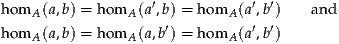
For the next two constructors of x, all but the first constructor
for y is likewise trivial. When x varies along j(1a) = reflia and y is
ib, we use the identity axiom again. Similarly, when x varies along
j(g∘f) = j(f) ▪j(g), we use associativity again. This completes the
construction of hom  :
:  0 →
0 → 0 →Set.
Step 2: We give the precategory structure on  , always by induction on
  0.
We are now eliminating into sets (the hom-sets of
0.
We are now eliminating into sets (the hom-sets of  ), so all but the first two
constructors are trivial to deal with.
), so all but the first two
constructors are trivial to deal with.
For identities, if x is ia then we have hom  (x, x) ≡ hom A(a, a) and
we define 1x :≡ 1ia. If x varies along je for e : a
(x, x) ≡ hom A(a, a) and
we define 1x :≡ 1ia. If x varies along je for e : a a′, we must show
that transportx
a′, we must show
that transportx hom
hom  (x,x)(je, 1ia) = 1ia
′. But by definition of hom
(x,x)(je, 1ia) = 1ia
′. But by definition of hom  ,
transporting along je is given by composing with e and e-1, and we have
e∘ 1ia ∘e-1 = 1ia′.
,
transporting along je is given by composing with e and e-1, and we have
e∘ 1ia ∘e-1 = 1ia′.
For composition, if x, y, z are ia, ib, ic respectively, then hom  reduces
to hom A and we can define composition in
reduces
to hom A and we can define composition in  to be composition in
A. And when x, y, or z varies along je, then we verify the following
equalities:
to be composition in
A. And when x, y, or z varies along je, then we verify the following
equalities:
| e∘ (g∘f) | = (e∘g) ∘f, | ||
| g∘f | = (g∘e-1) ∘ (e∘f), | ||
| (g∘f) ∘e-1 | = g∘ (f ∘e-1). |
Step 3: We show that  is a category. That is, we must show that for all
x, y :
is a category. That is, we must show that for all
x, y :  , the function idtoiso : (x = y) → (x
 y) is an equivalence. First we
define, for all x, y :
y) is an equivalence. First we
define, for all x, y :  , a function kx,y : (x
 y) → (x = y) by induction.
As before, since our goal is a set, it suffices to deal with the first two
constructors.
y) → (x = y) by induction.
As before, since our goal is a set, it suffices to deal with the first two
constructors.
When x and y are ia and ib respectively, we have hom  (ia, ib) ≡ hom A(a, b),
with composition and identities inherited as well, so that (ia
(ia, ib) ≡ hom A(a, b),
with composition and identities inherited as well, so that (ia ib) is
equivalent to (a
ib) is
equivalent to (a b). But now we have the constructor j : (a
 b) → (ia = ib).
Next, if y varies along j(e) for some e : b b′, we must show that for
f : a
b′, we must show that for
f : a b we have j(j(e)*
 ) = j(f) ▪j(e). But by definition of hom
  on
equalities, transporting along j(e) is equivalent to post-composing with e, so
this equality follows from the last constructor of
on
equalities, transporting along j(e) is equivalent to post-composing with e, so
this equality follows from the last constructor of  0. The remaining case when
x varies along j(e) for e : a
0. The remaining case when
x varies along j(e) for e : a a′ is similar. This completes the definition of
k : ∏(x,y: ^A
0) (x
a′ is similar. This completes the definition of
k : ∏(x,y: ^A
0) (x y) → (x = y).
Now one thing we must show is that if p : x = y, then k(idtoiso(p)) = p.
By induction on p, we may assume it is reflx, and hence idtoiso(p) ≡ 1x. Now
we argue by induction on x :  0, and since our goal is a mere proposition
(since
0, and since our goal is a mere proposition
(since  0 is a 1-type), all constructors except the first are trivial. But if x is ia,
then k(1ia) ≡ j(1a), which is equal to reflia by the third constructor of
0 is a 1-type), all constructors except the first are trivial. But if x is ia,
then k(1ia) ≡ j(1a), which is equal to reflia by the third constructor of
 0.
0.
To complete the proof that  is a category, we must show that if f : x
 y,
then idtoiso(k(f)) = f. By induction we may assume that x and y are ia and ib
respectively, in which case f must arise from an isomorphism g : a
y,
then idtoiso(k(f)) = f. By induction we may assume that x and y are ia and ib
respectively, in which case f must arise from an isomorphism g : a b and we
have k(f) ≡ j(g). However, for any p we have idtoiso(p) = p*
b and we
have k(f) ≡ j(g). However, for any p we have idtoiso(p) = p* , so in
particular idtoiso(j(g)) = j(g)*
, so in
particular idtoiso(j(g)) = j(g)* . And by definition of hom
  on equalities,
this is given by composing 1ia with the equivalence g, hence is equal to
g.
on equalities,
this is given by composing 1ia with the equivalence g, hence is equal to
g.
Note the similarity of this step to the encode-decode method used in §§2.12
and 2.13 and Chapter 8. Once again we are characterizing the identity types
of a higher inductive type (here,  0) by defining recursively a family of codes
(here, (x, y)
0) by defining recursively a family of codes
(here, (x, y) (x
(x y)) and encoding and decoding functions by induction on
 0 and on paths.
Step 4: We define a weak equivalence I : A → . We take
I0 :≡ i : A0 →
. We take
I0 :≡ i : A0 → 0, and by construction of hom
  we have functions
Ia,b : hom A(a, b) → hom
we have functions
Ia,b : hom A(a, b) → hom  (Ia, Ib) forming a functor I : A →
 . This functor
is fully faithful by construction, so it remains to show it is essentially
surjective. That is, for all x :
. This functor
is fully faithful by construction, so it remains to show it is essentially
surjective. That is, for all x :  we want there to merely exist an a : A such that
Ia
we want there to merely exist an a : A such that
Ia x. As always, we argue by induction on x, and since the goal is a mere
proposition, all but the first constructor are trivial. But if x is ia, then of course
we have a : A and Ia ≡ ia, hence Ia
x. As always, we argue by induction on x, and since the goal is a mere
proposition, all but the first constructor are trivial. But if x is ia, then of course
we have a : A and Ia ≡ ia, hence Ia ia. (Note that if we were trying to prove
I to be split essentially surjective, we would be stuck, because we know
nothing about equalities in A0 and thus have no way to deal with any further
constructors.) __
ia. (Note that if we were trying to prove
I to be split essentially surjective, we would be stuck, because we know
nothing about equalities in A0 and thus have no way to deal with any further
constructors.) __
We call the construction A
 the Rezk completion, although there is
also an argument (coming from higher topos semantics) for calling it the stack
completion.
the Rezk completion, although there is
also an argument (coming from higher topos semantics) for calling it the stack
completion.
We have seen that most precategories arising in practice are categories,
since they are constructed from et, which is a category by the univalence
axiom. However, there are a few cases in which the Rezk completion is
necessary to obtain a category.
Example 9.9.6. Recall from Example 9.1.17 that for any type X there is
a pregroupoid with X as its type of objects and hom(x, y) :≡ 0.
Its Rezk completion is the fundamental groupoid of X. Recalling that
groupoids are equivalent to 1-types, it is not hard to identify this
groupoid with
0.
Its Rezk completion is the fundamental groupoid of X. Recalling that
groupoids are equivalent to 1-types, it is not hard to identify this
groupoid with  1.
1.
Example 9.9.7. Recall from Example 9.1.18 that there is a precategory
whose type of objects is and with hom(X, Y) :≡ 0. Its Rezk
completion may be called the homotopy category of types. Its type of
objects can be identified with
0. Its Rezk
completion may be called the homotopy category of types. Its type of
objects can be identified with  1 (see Exercise 9.9).
The Rezk completion also allows us to show that the notion of “category” is determined by the notion of “weak equivalence of precategories”. Thus, insofar as the latter is inevitable, so is the former.
Theorem 9.9.8. A precategory C is a category if and only if for every weak equivalence of precategories H : A → B, the induced functor (– ∘H) : CB → CA is an isomorphism of precategories.
Proof. “Only if” is Theorem 9.9.4. In the other direction, let H be I : A →
 . Then since (– ∘I)0 is an equivalence, there exists R :
  → A such
that RI = 1A. Hence IRI = I, but again since (– ∘I)0 is an equivalence,
this implies IR = 1
→ A such
that RI = 1A. Hence IRI = I, but again since (– ∘I)0 is an equivalence,
this implies IR = 1 . By Lemma 9.4.9(iii), I is an isomorphism of
precategories. But then since
. By Lemma 9.4.9(iii), I is an isomorphism of
precategories. But then since  is a category, so is A. __
The original definition of categories, of course, was in set-theoretic foundations, so that the collection of objects of a category formed a set (or, for large categories, a class). Over time, it became clear that all “category-theoretic” properties of objects were invariant under isomorphism, and that equality of objects in a category was not usually a very useful notion. Numerous authors [Bla79, Fre76, Mak95, Mak01] discovered that a dependently typed logic enabled formulating the definition of category without invoking any notion of equality for objects, and that the statements provable in this logic are precisely the “category-theoretic” ones that are invariant under isomorphism.
Although most of category theory appears to be invariant under isomorphism of objects and under equivalence of categories, there are some interesting exceptions, which have led to philosophical discussions about what it means to be “category-theoretic”. For instance, Example 9.6.3 was brought up by Peter May on the categories mailing list in May 2010, as a case where it matters that two categories (defined as usual in set theory) are isomorphic rather than only equivalent. The case of †-categories was also somewhat confounding to those advocating an isomorphism-invariant version of category theory, since the “correct” notion of sameness between objects of a †-category is not ordinary isomorphism but unitary isomorphism.
Categories satisfying the “saturation” or “univalence” principle as in Definition 9.1.6 were first considered by Hofmann and Streicher [HS98]. The condition then occurred independently to Voevodsky, Shulman, and perhaps others around the same time several years later, and was formalized by Ahrens and Kapulkin [AKS13]. This framework puts all the above examples in a unified context: some precategories are categories, others are strict categories, and so on. A general theorem that “isomorphism implies equality” for a large class of algebraic structures (assuming the univalence axiom) was proven by Coquand and Danielsson; the formulation of the structure identity principle in §9.8 is due to Aczel.
Independently of philosophical considerations about category theory, Rezk [Rez01] discovered that when defining a notion of (∞, 1)-category, it was very convenient to use not merely a set of objects with spaces of morphisms between them, but a space of objects incorporating all the equivalences and homotopies between them. This yields a very well-behaved sort of model for (∞, 1)-categories as particular simplicial spaces, which Rezk called complete Segal spaces. One especially good aspect of this model is the analogue of Lemma 9.4.14: a map of complete Segal spaces is an equivalence just when it is a levelwise equivalence of simplicial spaces.
When interpreted in Voevodsky’s simplicial set model of univalent foundations, our precategories are similar to a truncated analogue of Rezk’s “Segal spaces”, while our categories correspond to his “complete Segal spaces”. Strict categories correspond instead to (a weakened and truncated version of) what are called “Segal categories”. It is known that Segal categories and complete Segal spaces are equivalent models for (∞, 1)-categories (see e.g. [Ber09]), so that in the simplicial set model, categories and strict categories yield “equivalent” category theories—although as we have seen, the former still have many advantages. However, in the more general categorical semantics of a higher topos, a strict category corresponds to an internal category (in the traditional sense) in the corresponding 1-topos of sheaves, while a category corresponds to a stack. The latter are generally a more appropriate sort of “category” relative to a topos.
In Rezk’s context, what we have called the “Rezk completion” corresponds to fibrant replacement in the model category for complete Segal spaces. Since this is built using a transfinite induction argument, it most closely matches our second construction as a higher inductive type. However, in higher topos models of homotopy type theory, the Rezk completion corresponds to stack completion, which can be constructed either with a transfinite induction [JT91] or using a Yoneda embedding [Bun79].
Exercise 9.1. For a precategory A and a : A, define the slice precategory A/a. Show that if A is a category, so is A/a.
Exercise 9.2. For any set X, prove that the slice category et/X is
equivalent to the functor category etX, where in the latter case we
regard X as a discrete category.
Exercise 9.3. Prove that a functor is an equivalence of categories if and only if it is a right adjoint whose unit and counit are isomorphisms.
Exercise 9.4. Define the notion of pre-2-category. Show that precategories, functors, and natural transformations as defined in §9.2 form a pre-2-category. Similarly, define a pre-bicategory by replacing the equalities (such as those in Lemmas 9.2.9 and 9.2.11) with natural isomorphisms satisfying analogous coherence conditions. Define a function from pre-2-categories to pre-bicategories, and show that it becomes an equivalence when restricted and corestricted to those whose hom-precategories are categories.
Exercise 9.5. Define a 2-category to be a pre-2-category satisfying
a condition analogous to that of Definition 9.1.6. Verify that the
pre-2-category of categories  at is a 2-category. How much of this
chapter can be done internally to an arbitrary 2-category?
at is a 2-category. How much of this
chapter can be done internally to an arbitrary 2-category?
Exercise 9.6. Define a 2-category whose objects are 1-types, whose
morphisms are functions, and whose 2-morphisms are homotopies.
Prove that it is equivalent, in an appropriate sense, to the full
sub-2-category of at spanned by the groupoids (categories in which
every arrow is an isomorphism).
Exercise 9.7. Recall that a strict category is a precategory whose type of objects is a set. Prove that the pre-2-category of strict categories is equivalent to the following pre-2-category.
Exercise 9.8. Define the pre-2-category of †-categories, which has †-structures on its hom-precategories. Show that two †-categories are equal precisely when they are “unitarily equivalent” in a suitable sense.
Exercise 9.9. Prove that a function X → Y is an equivalence if and only if
its image in the homotopy category of Example 9.9.7 is an isomorphism.
Show that the type of objects of this category is  1.
1.
Exercise 9.10. Construct the †-Rezk completion of a †-precategory into a †-category, and give it an appropriate universal property.
Exercise 9.11. Using fundamental (pre)groupoids from Examples 9.1.17 and 9.9.6 and the Rezk completion from §9.9, give a different proof of van Kampen’s theorem (§8.7).
Exercise 9.12. Let X and Y be sets and p : Y → X a surjection.
Our conception of sets as types with particularly simple homotopical character, cf. §3.1, is quite different from the sets of Zermelo–Fraenkel set theory, which form a cumulative hierarchy with an intricate nested membership structure. For many mathematical purposes, the homotopy-theoretic sets are just as good as the Zermelo–Fraenkel ones, but there are important differences.
We begin this chapter in §10.1 by showing that the category et has (most
of) the usual properties of the category of sets. In constructive, predicative,
univalent foundations, it is a “ΠW-pretopos”; whereas if we assume
propositional resizing (§3.5) it is an elementary topos, and if we assume
LEM and AC then it is a model of Lawvere’s Elementary Theory of the
Category of Sets. This is sufficient to ensure that the sets in homotopy type
theory behave like sets as used by most mathematicians outside of set
theory.
In the rest of the chapter, we investigate some subjects that traditionally belong to “set theory”. In §§10.2–10.4 we study cardinal and ordinal numbers. These are traditionally defined in set theory using the global membership relation, but we will see that the univalence axiom enables an equally convenient, more “structural” approach.
Finally, in §10.5 we consider the possibility of constructing inside of homotopy type theory a cumulative hierarchy of sets, equipped with a binary membership relation akin to that of Zermelo–Fraenkel set theory. This combines higher inductive types with ideas from the field of algebraic set theory.
In this chapter we will often use the traditional logical notation described in §3.7. In addition to the basic theory of Chapters 2 and 3, we use higher inductive types for colimits and quotients as in §§6.8 and 6.10, as well as some of the theory of truncation from Chapter 7, particularly the factorization system of §7.6 in the case n = -1. In §10.3 we use an inductive family (§5.7) to describe well-foundedness, and in §10.5 we use a more complicated higher inductive type to present the cumulative hierarchy.
Recall that in Chapter 9 we defined the category et to consist of all 0-types
(in some universe ) and maps between them, and observed that it is a
category (not just a precategory). We consider successively the levels of
structure which et possesses.
Since sets are closed under products, the universal property of products in
Theorem 2.15.2 shows immediately that et has finite products. In fact,
infinite products follow just as easily from the equivalence
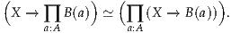
And we saw in Exercise 2.11 that the pullback of f : A → C and g : B → C
can be defined as ∑(a:A) ∑(b:B) f(a) = g(b); this is a set if A, B, C are and
inherits the correct universal property. Thus, et is a complete category in the
obvious sense.
Since sets are closed under + and contain 0, et has finite coproducts.
Similarly, since ∑(a:A) B(a) is a set whenever A and each B(a) are, it yields a
coproduct of the family B in et. Finally, we showed in §7.4 that pushouts
exist in n-types, which includes et in particular. Thus, et is also cocomplete.
Next, we show that et is a regular category, i.e.:
et is finitely complete.
Recall that a regular epimorphism is a morphism that is the coequalizer of some pair of maps. Thus in (iii) the pullback of a coequalizer is required to again be a coequalizer, but not necessarily of the pulled-back pair.
The obvious candidate for the coequalizer of the kernel pair of
f : A → B is the image of f, as defined in §7.6. Recall that we defined
im(f) :≡ ∑(b:B)  , with functions
  : A →im(f) and if : im(f) → B
defined by
: A →im(f) and if : im(f) → B
defined by
 | :≡ λa.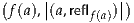 | ||
| if | :≡pr1 |
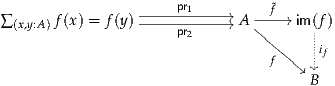 |
Recall that a function f : A → B is called surjective if
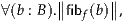 |
or equivalently ∀(b : B).∃(a : A).f(a) = b. We have also said that a function
f : A → B between sets is called injective if ∀(a, a′ : A).(f(a) = f(a′)) ⇒ (a = a′),
or equivalently if each of its fibers is a mere proposition. Since these are the
(-1)-connected and (-1)-truncated maps in the sense of Chapter 7, the
general theory there implies that  above is surjective and if is injective, and
that this factorization is stable under pullback.
above is surjective and if is injective, and
that this factorization is stable under pullback.
We now identify surjectivity and injectivity with the appropriate category-theoretic notions. First we observe that categorical monomorphisms and epimorphisms have a slightly stronger equivalent formulation.
Lemma 10.1.1. For a morphism f : hom A(a, b) in a category A, the following are equivalent.
Proof. The equivalence of conditions (i) and (ii) is standard category theory. Now consider the function (f ∘ –) : hom A(x, a) → hom A(x, b) between sets. Condition (i) says that it is injective, while (iii) says that its fibers are mere propositions; hence they are equivalent. And (iii) implies (iv) by taking k :≡ f ∘g and recalling that an inhabited mere proposition is contractible. Finally, (iv) implies (i) since if p : f ∘g = f ∘h, then (g, refl) and (h, p) both inhabit the type in (iv), hence are equal and so g = h. __
Lemma 10.1.2. A function f : A → B between sets is injective if and only if
it is a monomorphism in et.
Proof. Left to the reader. __
Of course, an epimorphism is a monomorphism in the opposite category.
We now show that in et, the epimorphisms are precisely the surjections, and
also precisely the coequalizers (regular epimorphisms).
The coequalizer of a pair of maps f, g : A → B in et is defined as the
0-truncation of a general (homotopy) coequalizer. For clarity, we may call this
the set-coequalizer. It is convenient to express its universal property as
follows.
Lemma 10.1.3. Let f, g : A → B be functions between sets A and B. The set-coequalizer cf,g : B → Qhas the property that, for any set C and any h : B → C with h∘f = h∘g, the type
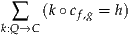 |
is contractible.
Proof. Let f : A → B be a function between sets, and suppose it to be an epimorphism; we show Cf is contractible. The constructor 1 → Cf of Cf gives us an element t : Cf. We have to show that
 |
Note that x = t is a mere proposition, hence we can use induction on Cf. Of course when x is t we have reflt : t = t, so it suffices to find
| I0 | : ∏ b:B ι(b) = t | ||
| I1 | : ∏ a:A α1(a)-1 ▪I 0(f(a)) = reflt. |
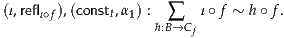 |
By the dual of Lemma 10.1.1(iv) (and function extensionality), there is a path
 |
Hence, we may define I0(b) :≡happly(appr1 (γ), b) : ι(b) = t. We also have

This transport involves precomposition with f, which commutes with happly. Thus, from transport in path types we obtain I0(f(a)) = α1(a) for any a : A, which gives us I1.
Now suppose Cf is contractible; we show f is surjective. We first construct a type family P : Cf →Prop by recursion on Cf, which is valid since Prop is a set. On the point constructors, we define
| P(t) | :≡1 | ||
| P(ι(b)) | :≡ . . |
 |
for all a : A. However,  is inhabited by (f(a), reflf(a)). Since it is a
mere proposition, this means it is contractible — and thus equivalent, hence
equal, to 1. This completes the definition of P. Now, since Cf is assumed to be
contractible, it follows that P(x) is equivalent to P(t) for any x : Cf. In
particular, P(ι(b)) ≡
is inhabited by (f(a), reflf(a)). Since it is a
mere proposition, this means it is contractible — and thus equivalent, hence
equal, to 1. This completes the definition of P. Now, since Cf is assumed to be
contractible, it follows that P(x) is equivalent to P(t) for any x : Cf. In
particular, P(ι(b)) ≡ is equivalent to P(t) ≡1 for each b : B, and
hence contractible. Thus, f is surjective.
is equivalent to P(t) ≡1 for each b : B, and
hence contractible. Thus, f is surjective.
Finally, suppose f : A → B to be surjective, and consider a set C and two
functions g, h : B → C with the property that g∘f = h∘f. Since f is assumed
to be surjective, for all b : B the type  is contractible. Thus we have
the following equivalences:
is contractible. Thus we have
the following equivalences:
| ∏ b:B (g(b) = h(b)) | ≃ ∏
b:B   → (g(b) = h(b)) → (g(b) = h(b)) | ||
≃ ∏
b:B  fibf(b) → (g(b) = h(b)) fibf(b) → (g(b) = h(b)) | |||
| ≃ ∏ (b:B) ∏ (a:A) ∏ (p:f(a)=b) g(b) = h(b) | |||
| ≃ ∏ a:A g(f(a)) = h(f(a)) |
Theorem 10.1.5. The category et is regular. Moreover, surjective functions
between sets are regular epimorphisms.
Proof. It is a standard lemma in category theory that a category is
regular as soon as it admits finite limits and a pullback-stable orthogonal
factorization system ( ,
,  ) with the monomorphisms, in which case
consists automatically of the regular epimorphisms. (See e.g. [Joh02,
A1.3.4].) The existence of the factorization system was proved in
Theorem 7.6.6. __
) with the monomorphisms, in which case
consists automatically of the regular epimorphisms. (See e.g. [Joh02,
A1.3.4].) The existence of the factorization system was proved in
Theorem 7.6.6. __
Proof. We showed in Theorem 7.6.9 that pullbacks of n-connected functions are n-connected. By Theorem 10.1.5, it suffices to apply this when n = -1. __
One of the consequences of et being a regular category is that we have an
“image” operation on subsets. That is, given f : A → B, any subset
P :  (A) (i.e. a predicate P : A →Prop) has an image which is a subset of
B. This can be defined directly as
(A) (i.e. a predicate P : A →Prop) has an image which is a subset of
B. This can be defined directly as  ∃(x : A).f(x) = y∧P(x)},
or indirectly as the image (in the previous sense) of the composite
function
∃(x : A).f(x) = y∧P(x)},
or indirectly as the image (in the previous sense) of the composite
function
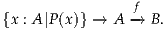
We will also sometimes use the common notation  P(x)} for the image
of P.
P(x)} for the image
of P.
Now that we know that et is regular, to show that et is exact, we need to
show that every equivalence relation is effective. In other words, given an
equivalence relation R : A → A →Prop, there is a coequalizer cR of the pair
pr1, pr2 : ∑(x,y:A) R(x, y) → A and, moreover, the pr1 and pr2 form the kernel
pair of cR.
We have already seen, in §6.10, two general ways to construct the quotient of a set by an equivalence relation R : A → A →Prop. The first can be described as the set-coequalizer of the two projections
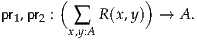
The important property of such a quotient is the following.
Since the standard pullback of cR and itself is ∑(x,y:A) (cR(x) = cR(y)), by Theorem 4.7.7 this is equivalent to asking that the canonical transformation ∏ (x,y:A) R(x, y) → (cR(x) = cR(y)) be a fiberwise equivalence.
Lemma 10.1.8. Suppose (A, R) is an equivalence relation. Then there is an equivalence
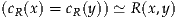 |
for any x, y : A. In other words, equivalence relations are effective.
Proof. We begin by extending R to a relation  : A/R → A/R →Prop,
which we will then show is equivalent to the identity type on A/R.
We define
: A/R → A/R →Prop,
which we will then show is equivalent to the identity type on A/R.
We define  by double induction on A/R (note that Prop is a set by
univalence for mere propositions). We define
by double induction on A/R (note that Prop is a set by
univalence for mere propositions). We define  (cR(x), cR(y)) :≡ R(x, y).
For r : R(x, x′) and s : R(y, y′), the transitivity and symmetry of R gives
an equivalence from R(x, y) to R(x′, y′). This completes the definition of
(cR(x), cR(y)) :≡ R(x, y).
For r : R(x, x′) and s : R(y, y′), the transitivity and symmetry of R gives
an equivalence from R(x, y) to R(x′, y′). This completes the definition of
 .
.
It remains to show that  (w, w′) ≃ (w = w′) for every w, w′ :
A/R. The direction (w = w′) →
(w, w′) ≃ (w = w′) for every w, w′ :
A/R. The direction (w = w′) →  (w, w′) follows by transport once
we show that
(w, w′) follows by transport once
we show that  is reflexive, which is an easy induction. The other
direction
is reflexive, which is an easy induction. The other
direction  (w, w′) → (w = w′) is a mere proposition, so since cR :
A → A/R is surjective, it suffices to assume that w and w′ are of
the form cR(x) and cR(y). But in this case, we have the canonical
map
(w, w′) → (w = w′) is a mere proposition, so since cR :
A → A/R is surjective, it suffices to assume that w and w′ are of
the form cR(x) and cR(y). But in this case, we have the canonical
map  (cR(x), cR(y)) :≡ R(x, y) → (cR(x) = cR(y)). (Note again the
appearance of the encode-decode method.) __
(cR(x), cR(y)) :≡ R(x, y) → (cR(x) = cR(y)). (Note again the
appearance of the encode-decode method.) __
The second construction of quotients is as the set of equivalence classes of R (a subset of its power set):

This requires propositional resizing in order to remain in the same universe as A and R.
Note that if we regard R as a function from A to A →Prop, then A⫽//R is equivalent to im(R), as constructed in §10.1.2. Now in Theorem 10.1.5 we have shown that images are coequalizers. In particular, we immediately get the coequalizer diagram
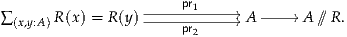 |
We can use this to give an alternative proof that any equivalence relation is effective and that the two definitions of quotients agree.
Theorem 10.1.9. For any function f : A → B between any two sets, the relation ker(f) : A → A →Prop given by ker(f, x, y) :≡ (f(x) = f(y)) is effective.
Proof. We will use that im(f) is the coequalizer of pr1, pr2 : ( ∑(x,y:A) f(x) = f(y)) → A. Note that the kernel pair of the function
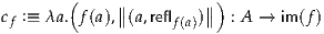
consists of the two projections
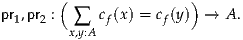 |
For any x, y : A, we have equivalences
| (cf(x) = cf(y)) | ≃ ∑
p:f(x)=f(y) p* ∑
p:f(x)=f(y) p*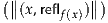 = =   | ||
| ≃ (f(x) = f(y)), |
 is a mere proposition for
any b : B. Therefore, we get that
is a mere proposition for
any b : B. Therefore, we get that
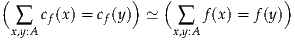 |
and hence we may conclude that ker f is an effective relation for any function f. __
Proof. We need to analyze the coequalizer diagram
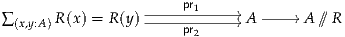 |
By the univalence axiom, the type R(x) = R(y) is equivalent to the type of homotopies from R(x) to R(y), which is equivalent to
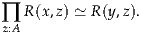 |
Since R is an equivalence relation, the latter space is equivalent to R(x, y). To summarize, we get that (R(x) = R(y)) ≃ R(x, y), so R is effective since it is equivalent to an effective relation. Also, the diagram
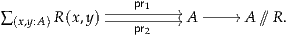 " class="math-display" >
 |
is a coequalizer diagram. Since coequalizers are unique up to equivalence, it follows that A/R ≃ A⫽//R. __
We finish this section by mentioning a possible third construction of the quotient of a set A by an equivalence relation R. Consider the precategory with objects A and hom-sets R; the type of objects of the Rezk completion (see §9.9) of this precategory will then be the quotient. The reader is invited to check the details.
et is a ΠW-pretoposThe notion of a ΠW-pretopos — that is, a locally cartesian closed category with disjoint finite coproducts, effective equivalence relations, and initial algebras for polynomial endofunctors — is intended as a “predicative” notion of topos, i.e. a category of “predicative sets”, which can serve the purpose for constructive mathematics that the usual category of sets does for classical mathematics.
Typically, in constructive type theory, one resorts to an external construction of “setoids” — an exact completion — to obtain a category with such closure properties. In particular, the well-behaved quotients are required for many constructions in mathematics that usually involve (non-constructive) power sets. It is noteworthy that univalent foundations provides these constructions internally (via higher inductive types), without requiring such external constructions. This represents a powerful advantage of our approach, as we shall see in subsequent examples.
Proof. We have an initial object 0 and finite, disjoint sums A + B.
These are stable under pullback, simply because pullback has a right
adjoint. Indeed, et is locally cartesian closed, since for any map f :
A → B between sets, the “fibrant replacement” ∑(a:A) f(a) = b is
equivalent to A (over B), and we have dependent function types for
the replacement. We’ve just shown that et is regular (Theorem 10.1.5)
and that quotients are effective (Lemma 10.1.8). We thus have a locally
cartesian closed pretopos. Finally, since the n-types are closed under the
formation of W-types by Exercise 7.3, and by Theorem 5.4.7 W-types
are initial algebras for polynomial endofunctors, we see that et is a
ΠW-pretopos. __
One naturally wonders what, if anything, prevents et from being an
(elementary) topos? In addition to the structure already mentioned, a topos
has a subobject classifier: a pointed object classifying (equivalence classes of)
monomorphisms. (In fact, in the presence of a subobject classifier, things
become somewhat simpler: one merely needs cartesian closure in order to get
the colimits.) In homotopy type theory, univalence implies that the type
Prop :≡ ∑(X:) isProp(X) does classify monomorphisms (by an argument
similar to §4.8), but in general it is as large as the ambient universe . Thus, it
is a “set” in the sense of being a 0-type, but it is not “small” in the sense of
being an object of , hence not an object of the category et. However, if we
assume an appropriate form of propositional resizing (see §3.5), then we
can find a small version of Prop, so that et becomes an elementary
topos.
Theorem 10.1.12. If there is a type Ω : of all mere propositions, then the
category etis an elementary topos.
A sufficient condition for this is the law of excluded middle, in the “mere-propositional” form that we have called LEM; for then we have Prop = 2, which is small, and which then also classifies all mere propositions. Moreover, in topos theory a well-known sufficient condition for LEM is the axiom of choice, which is of course often assumed as an axiom in classical set theory. In the next section, we briefly investigate the relation between these conditions in our setting.
We begin with the following lemma.
Lemma 10.1.13. If A is a mere proposition then its suspension Σ(A) is a set, and Ais equivalent to N =Σ(A) S.
Proof. To show that Σ(A) is a set, we define a family P : Σ(A) → Σ(A) →
with the property that P(x, y) is a mere proposition for each x, y : Σ(A), and
which is equivalent to its identity type IdΣ(A). We make the following
definitions:
| P(N, N) | :≡1 | P(S, N) | :≡ A | ||||
| P(N, S) | :≡ A | P(S, S) | :≡1. |
 |
But since A is inhabited by a, it is equivalent to 1, so we have
 |
The univalence axiom turns these into the desired equalities. Also, P(x, y) is a mere proposition for all x, y : Σ(A), which is proved by induction on x and y, and using the fact that being a mere proposition is a mere proposition.
Note that P is a reflexive relation. Therefore we may apply Theorem 7.2.2, so it suffices to construct τ : ∏(x,y:Σ(A)) P(x, y) → (x = y). We do this by a double induction. When x is N, we define τ(N) by
 |
If A is inhabited by a then merid(a) : N = S so we also need
 |
This we get by function extensionality using the fact that, for all x : A,
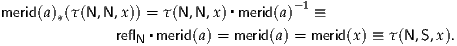 |
 |
To complete the construction of τ, we need to check merid(a)* = τ(S),
given any a : A. The verification proceeds much along the same lines by
induction on the second argument of τ.
= τ(S),
given any a : A. The verification proceeds much along the same lines by
induction on the second argument of τ.
Thus, by Theorem 7.2.2 we have that Σ(A) is a set and that P(x, y) ≃ (x = y) for all x, y : Σ(A). Taking x :≡N and y :≡S yields A ≃ (N =Σ(A) S) as desired. __
Proof. We use the equivalent form of choice given in Lemma 3.8.2.
Consider a mere proposition A. The function f : 2 → Σ(A) defined by
f(02) :≡ N and f(12) :≡ S is surjective. Indeed, we have (02, reflN) :
fibf(N) and (12, reflS) : fibf(S). Since  fibf(x)
 is a mere proposition, by
induction the claimed surjectivity follows.
is a mere proposition, by
induction the claimed surjectivity follows.
By Lemma 10.1.13 the suspension Σ(A) is a set, so by the axiom of choice there merely exists a section g : Σ(A) →2 of f. As equality on 2 is decidable we get
 |
and, since g is a section of f, hence injective,
 |
Finally, since (f(02) = f(12)) = (N = S) = A by Lemma 10.1.13, we have A + ¬A. __
Theorem 10.1.15. If the axiom of choice holds then the category et is a
well-pointed boolean elementary topos with choice.
Proof. Since AC implies LEM, we have a boolean elementary topos with choice by Theorem 10.1.12 and the remark following it. We leave the proof of well-pointedness as an exercise for the reader (Exercise 10.3). __
Remark 10.1.16. The conditions on a category mentioned in the theorem are known as Lawvere’s axioms for the Elementary Theory of the Category of Sets [Law05].
Definition 10.2.1. The type of cardinal numbers is the 0-truncation of the type Set of sets:
Thus, a cardinal number, or cardinal, is an inhabitant of Card ≡ 0.
Technically, of course, there is a separate type Card associated to each
universe .
0.
Technically, of course, there is a separate type Card associated to each
universe .
As usual for truncations, if A is a set, then  0 denotes its image under the
canonical projection Set →
0 denotes its image under the
canonical projection Set → 0 ≡Card; we call
  0 the cardinality of A.
By definition, Card is a set. It also inherits the structure of a semiring from
Set.
0 the cardinality of A.
By definition, Card is a set. It also inherits the structure of a semiring from
Set.
Proof. Since Card → Card is a set, to define (α + –) : Card → Card for
all α : Card, by induction it suffices to assume that α is  0 for some
A : Set. Now we want to define (
0 for some
A : Set. Now we want to define ( 0 + –) : Card →Card, i.e. we want
to define
0 + –) : Card →Card, i.e. we want
to define  0 + β : Card for all β : Card. However, since Card is a set, by
induction it suffices to assume that β is
0 + β : Card for all β : Card. However, since Card is a set, by
induction it suffices to assume that β is  0 for some B : Set. But now
we can define
0 for some B : Set. But now
we can define  0 +
0 +  0 to be
  0. __
0. __
Definition 10.2.3. Similarly, the operation of cardinal multiplication

is defined by induction on truncation:
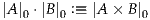
Lemma 10.2.4. Card is a commutative semiring, i.e. for α, β, γ : Card we have the following.
| (α + β) + γ | = α + (β + γ) | ||
| α + 0 | = α | ||
| α + β | = β + α | ||
| (α⋅β) ⋅γ | = α⋅ (β⋅γ) | ||
| α⋅ 1 | = α | ||
| α⋅β | = β⋅α | ||
| α⋅ (β + γ) | = α⋅β + α⋅γ |
 0 and 1 :≡
 0.
0.
Proof. We prove the commutativity of multiplication, α⋅β = β⋅α; the
others are exactly analogous. Since Card is a set, the type α⋅β = β⋅α is
a mere proposition, and in particular a set. Thus, by induction it suffices
to assume α and β are of the form  0 and
0 and  0 respectively, for some
A, B : Set. Now
0 respectively, for some
A, B : Set. Now  0 ⋅
0 ⋅ 0 ≡
0 ≡ 0 and
0 and  0 ×
0 × 0 ≡
0 ≡ 0,
so it suffices to show A×B = B×A. Finally, by univalence, it suffices to
give an equivalence A×B ≃ B×A. But this is easy: take (a, b)
0,
so it suffices to show A×B = B×A. Finally, by univalence, it suffices to
give an equivalence A×B ≃ B×A. But this is easy: take (a, b) (b, a)
and its obvious inverse. __
(b, a)
and its obvious inverse. __
Definition 10.2.5. The operation of cardinal exponentiation is also defined by induction on truncation:
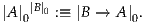
Lemma 10.2.6. For α, β, γ : Card we have
| α0 | = 1 | ||
| 1α | = 1 | ||
| α1 | = α | ||
| αβ+γ | = αβ ⋅αγ | ||
| αβ⋅γ | = (αβ)γ | ||
| (α⋅β)γ | = αγ ⋅βγ |
Proof. Exactly like Lemma 10.2.4. __
Definition 10.2.7. The relation of cardinal inequality

is defined by induction on truncation:
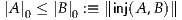
where inj(A, B) is the type of injections from A to B. In other words,
 0 ≤
0 ≤ 0 means that there merely exists an injection from A to B.
Proof. As before, by induction on truncation. For instance, since (α ≤
β) → (β ≤ γ) → (α ≤ γ) is a mere proposition, by induction
on 0-truncation we may assume α, β, and γ are  0,
0,  0, and
  0
respectively. Now since
0
respectively. Now since  0 ≤
0 ≤ 0 is a mere proposition, by induction
on (-1)-truncation we may assume given injections f : A → B and
g : B → C. But then g∘f is an injection from A to C, so
0 is a mere proposition, by induction
on (-1)-truncation we may assume given injections f : A → B and
g : B → C. But then g∘f is an injection from A to C, so  0 ≤
0 ≤ 0
holds. Reflexivity is even easier. __
0
holds. Reflexivity is even easier. __
We may likewise show that cardinal inequality is compatible with the semiring operations.
Proof. If f : A → B is an injection, define g : B → A at b : B as follows. Since f is injective, the fiber of f at b is a mere proposition. Therefore, by excluded middle, either there is an a : A with f(a) = b, or not. In the first case, define g(b) :≡ a; otherwise set g(b) :≡ a0. Then for any a : A, we have a = g(f(a)), so g is surjective.
The second statement follows from this by induction on truncation. For the third, if g : B → A is surjective, then by the axiom of choice, there merely exists a function f : A → B with g(f(a)) = a for all a. But then f must be injective. __
Proof. The usual “back-and-forth” argument applies without significant
changes. Note that it actually constructs an isomorphism A B
(assuming excluded middle so that we can decide whether a given
element belongs to a cycle, an infinite chain, a chain beginning in A, or a
chain beginning in B). __
B
(assuming excluded middle so that we can decide whether a given
element belongs to a cycle, an infinite chain, a chain beginning in A, or a
chain beginning in B). __
Corollary 10.2.11. Assuming excluded middle, cardinal inequality is a partial order, i.e. for α, β : Card we have

Proof. Since α = β is a mere proposition, by induction on truncation we
may assume α and β are  0 and
0 and  0, respectively, and that we have
injections f : A → B and g : B → A. But then the Schroeder–Bernstein
theorem gives an isomorphism A ≃ B, hence an equality
0, respectively, and that we have
injections f : A → B and g : B → A. But then the Schroeder–Bernstein
theorem gives an isomorphism A ≃ B, hence an equality  0 =
0 =
 0. __
0. __
Finally, we can reproduce Cantor’s theorem, showing that for every cardinal there is a greater one.
Proof. Suppose f : A → (A →2) is any function, and define g : A →2 by g(a) :≡¬f(a)(a). If g = f(a0), then g(a0) = f(a0)(a0) but g(a0) = ¬f(a0)(a0), a contradiction. Thus, f is not surjective. __
Corollary 10.2.13. Assuming excluded middle, for any α : Card, there is a cardinal βsuch that α ≤ βand α≠β.
Proof. Let β = 2α. Now we want to show a mere proposition, so by
induction we may assume α is  0, so that β ≡
  0. Using
excluded middle, we have a function f : A → (A →2) defined by
0. Using
excluded middle, we have a function f : A → (A →2) defined by
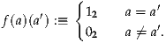
And if f(a) = f(a′), then f(a′)(a) = f(a)(a) = 12, so a = a′; hence f is
injective. Thus, α ≡ 0 ≤
0 ≤ 0 ≡ 2α.
On the other hand, if 2α ≤ α, then we would have an injection (A → 2) → A. By Lemma 10.2.9, since we have (λx.02) : A → 2 and excluded middle, there would then be a surjection A → (A →2), contradicting Cantor’s theorem. __
Definition 10.3.1. Let A be a set and
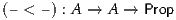
a binary relation on A. We define by induction what it means for an element a : A to be accessible by <:
We write acc(a) to mean that a is accessible.
It may seem that such an inductive definition can never get off the ground, but of course if a has the property that there are no b such that b < a, then a is vacuously accessible.
Note that this is an inductive definition of a family of types, like the type of vectors considered in §5.7. More precisely, it has one constructor, say acc<, with type
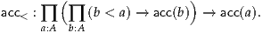
The induction principle for acc says that for any P : ∏(a:A) acc(a) →, if we
have

then we have g : ∏(a:A) ∏(c:acc(a)) P(a, c) defined by induction, with

This is a mouthful, but generally we apply it only in the simpler case
where P : A → depends only on A. In this case the second and
third arguments of f may be combined, so that what we have to prove
is
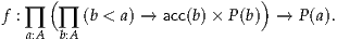
That is, we assume every b < a is accessible and g(b) : P(b) is defined, and from these define g(a) : P(a).
The omission of the second argument of P is justified by the following lemma, whose proof is the only place where we use the more general form of the induction principle.
Proof. We must show that for any a : A and s1, s2 : acc(a) we have s1 = s2. We prove this by induction on s1, with
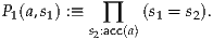
Thus, we must show that for any a : A and h1 : ∏(b:A) (b < a) →acc(b) and
we have acc<(a, h) = s2 for any s2 : acc(a). We regard this statement as ∏ (a:A) ∏(s2:acc(a)) P2(a, s2), where
thus we may prove it by induction on s2. Therefore, we assume h2 : ∏ (b:A) (b < a) →acc(b), and k2 with a monstrous but irrelevant type, and must show that for any h1 and k1 with types as above, we have acc<(a, h1) = acc<(a, h2). By function extensionality, it suffices to show h1(b, l) = h2(b, l) for all b : A and l : b < a. This follows from k1. __
Definition 10.3.3. A binary relation < on a set A is well-founded if every element of A is accessible.
The point of well-foundedness is that for P : A →, we can use the
induction principle of acc to conclude ∏(a:A) acc(a) → P(a), and then apply
well-foundedness to conclude ∏(a:A) P(a). In other words, if from
∀(b : A).(b < a) → P(b) we can prove P(a), then ∀(a : A).P(a). This is called
well-founded induction.
Proof. Well-foundedness of < is the type ∏(a:A) acc(a), which is a mere proposition since each acc(a) is. __
Example 10.3.5. Perhaps the most familiar well-founded relation is the usual strict ordering on N. To show that this is well-founded, we must show that n is accessible for each n : N. This is just the usual proof of “strong induction” from ordinary induction on N.
Specifically, we prove by induction on n : N that k is accessible for all k ≤ n. The base case is just that 0 is accessible, which is vacuously true since nothing is strictly less than 0. For the inductive step, we assume that k is accessible for all k ≤ n, which is to say for all k < n + 1; hence by definition n + 1 is also accessible.
A different relation on N which is also well-founded is obtained by setting only n < succ(n) for all n : N. Well-foundedness of this relation is almost exactly the ordinary induction principle of N.
Example 10.3.6. Let A : Set and B : A →Set be a family of sets. Recall from §5.3 that the W-type W(a:A)B(a) is inductively generated by the single constructor
We define the relation < on W(x:A)B(x) by recursion on its second argument:
Now we prove that every w : W(x:A)B(x) is accessible for this relation, using the usual induction principle for W(x:A)B(x). This means we assume given a : A and f : B(a) →W(x:A)B(x), and also a lifting f′ : ∏(b:B(a)) acc(f(b)). But then by definition of <, we have acc(w) for all w < sup(a, f); hence sup(a, f) is accessible.
Well-foundedness allows us to define functions by recursion and prove
statements by induction, such as for instance the following. Recall from §3.5
that (B) denotes the power set (B) :≡ (B →Prop).
Lemma 10.3.7. Suppose B is a set and we have a function

Then if <is a well-founded relation on A, there is a function f : A → B such that for all a : Awe have
 |
(We are using the notation for images of subsets from §10.1.2.)
Proof. We first define, for every a : A and s : acc(a), an element (a, s) : B. By induction, it suffices to assume that s is a function assigning to each a′ < a a witness s(a′) : acc(a′), and that moreover for each such a′ we have an element (a′, s(a′)) : B. In this case, we define
 |
Now since < is well-founded, we have a function w : ∏(a:A) acc(a). Thus, we can define f(a) :≡(a, w(a)). __
In classical logic, well-foundedness has a more well-known reformulation.
In the following, we say that a subset B : (A) is nonempty if it is unequal to
the empty subset (λx.⊥) : (X). We leave it to the reader to verify that
assuming excluded middle, this is equivalent to mere inhabitation, i.e. to the
condition ∃(x : A).x ∈ B.
Lemma 10.3.8. Assuming excluded middle, < is well-founded if and only if
every nonempty subset B : (A) merely has a minimal element.
Proof. Suppose first < is well-founded, and suppose B ⊆ A is a subset with no minimal element. That is, for any a : A with a ∈ B, there merely exists a b : A with b < a and b ∈ B.
We claim that for any a : A and s : acc(a), we have a B. By
induction, we may assume s is a function assigning to each a′ < a a proof
s(a′) : acc(a), and that moreover for each such a′ we have a′
B. By
induction, we may assume s is a function assigning to each a′ < a a proof
s(a′) : acc(a), and that moreover for each such a′ we have a′ B. If a ∈ B,
then by assumption, there would merely exist a b < a with b ∈ B, which
contradicts this assumption. Thus, a
B. If a ∈ B,
then by assumption, there would merely exist a b < a with b ∈ B, which
contradicts this assumption. Thus, a B; this completes the induction.
Since < is well-founded, we have a
B; this completes the induction.
Since < is well-founded, we have a B for all a : A, i.e. B is empty.
Now suppose each nonempty subset merely has a minimal element.
Let B =  ¬acc(a)}. Then if B is nonempty, it merely has a minimal
element. Thus there merely exists an a : A with a ∈ B such that for
all b < a, we have acc(b). But then by definition (and induction on
truncation), a is merely accessible, and hence accessible, contradicting
a ∈ B. Thus, B is empty, so < is well-founded. __
¬acc(a)}. Then if B is nonempty, it merely has a minimal
element. Thus there merely exists an a : A with a ∈ B such that for
all b < a, we have acc(b). But then by definition (and induction on
truncation), a is merely accessible, and hence accessible, contradicting
a ∈ B. Thus, B is empty, so < is well-founded. __
Note that since A is a set, extensionality is a mere proposition. This notion of “extensionality” is unrelated to function extensionality, and also unrelated to the extensionality of identity types. Rather, it is a “local” counterpart of the axiom of extensionality in classical set theory.
Proof. By the univalence axiom, it suffices to show that if (A, <) is
extensional and well-founded and f : (A, <) (A, <), then f = idA.
We prove by induction on < that f(a) = a for all a : A. The inductive
hypothesis is that for all a′ < a, we have f(a′) = a′.
(A, <), then f = idA.
We prove by induction on < that f(a) = a for all a : A. The inductive
hypothesis is that for all a′ < a, we have f(a′) = a′.
Now since A is extensional, to conclude f(a) = a it is sufficient to show

However, since f is an automorphism, we have (c < a) ⇔ (f(c) < f(a)). But c < a implies f(c) = c by the inductive hypothesis, so (c < a) → (c < f(a)). On the other hand, if c < f(a), then f-1(c) < a, and so c = f(f-1(c)) = f-1(c) by the inductive hypothesis again; thus c < a. Therefore, we have (c < a) ⇔ (c < f(a)) for any c : A, so f(a) = a. __
Definition 10.3.11. If (A, <) and (B, <) are extensional and well-founded, a simulation is a function f : A → B such that
Proof. We prove by double well-founded induction that for any a, b : A, if f(a) = f(b) then a = b. The inductive hypothesis for a : A says that for any a′ < a, and any b : B, if f(a′) = f(b) then a = b. The inner inductive hypothesis for b : A says that for any b′ < b, if f(a) = f(b′) then a = b′.
Suppose f(a) = f(b); we must show a = b. By extensionality, it suffices to show that for any c : A we have (c < a) ⇔ (c < b). If c < a, then f(c) < f(a) by Definition 10.3.11(i). Hence f(c) < f(b), so by Definition 10.3.11(ii) there merely exists c′ : A with c′ < b and f(c) = f(c′). By the inductive hypothesis for a, we have c = c′, hence c < b. The dual argument is symmetrical. __
In particular, this implies that in Definition 10.3.11(ii) the word “merely” could be omitted without change of sense.
Corollary 10.3.13. If f : A → B is a simulation, then for all a : A and b : B, if b < f(a), there purely exists an a′ < awith f(a′) = b.
Proof. Since f is injective, ∑(a:A) (f(a) = b) is a mere proposition. __
We say that a subset C : (B) is an initial segment if c ∈ C and b < c
imply b ∈ C. The image of a simulation must be an initial segment, while the
inclusion of any initial segment is a simulation. Thus, by univalence, every
simulation A → B is equal to the inclusion of some initial segment of
B.
Theorem 10.3.14. For a set A, let P(A) be the type of extensional
well-founded relations on A. If < A : P(A) and < B : P(B) and f : A → B,
let H<A<B(f) be the mere proposition that f is a simulation. Then (P, H) is a
standard notion of structure over etin the sense of §9.8.
Proof. We leave it to the reader to verify that identities are simulations, and that composites of simulations are simulations. Thus, we have a notion of structure. For standardness, we must show that if < and ≺ are two extensional well-founded relations on A, and idA is a simulation in both directions, then < and ≺ are equal. Since extensionality and well-foundedness are mere propositions, for this it suffices to have ∀(a, b : A).(a < b) ⇔ (a ≺ b). But this follows from Definition 10.3.11(i) for idA. __
Corollary 10.3.15. There is a category whose objects are sets equipped with extensional well-founded relations, and whose morphisms are simulations.
In fact, this category is a poset.
Lemma 10.3.16. For extensional and well-founded (A, <) and (B, <), there is at most one simulation f : A → B.
Proof. Suppose f, g : A → B are simulations. Since being a simulation is a mere property, it suffices to show ∀(a : A).(f(a) = g(a)). By induction on <, we may suppose f(a′) = g(a′) for all a′ < a. And by extensionality of B, to have f(a) = g(a) it suffices to have ∀(b : B).(b < f(a)) ⇔ (b < g(a)).
But since f is a simulation, if b < f(a), then we have a′ < a with f(a′) = b. By the inductive hypothesis, we have also g(a′) = b, hence b < g(a). The dual argument is symmetrical. __
Thus, if A and B are equipped with extensional and well-founded relations, we may write A ≤ B to mean there exists a simulation f : A → B. Corollary 10.3.15 implies that if A ≤ B and B ≤ A, then A = B.
Definition 10.3.17. An ordinal is a set A with an extensional well-founded relation which is transitive, i.e. satisfies ∀(a, b, c : A).(a < b) → (b < c) → (a < c).
Example 10.3.18. Of course, the usual strict order on N is transitive. It is easily seen to be extensional as well; thus it is an ordinal. As usual, we denote this ordinal by ω.
Let Ord denote the type of ordinals. By the previous results, Ord is a set and has a natural partial order. We now show that Ord also admits a well-founded relation.
If A is an ordinal and a : A, let A/a :≡ b < a} denote the initial
segment. Note that if A/a = A/b as ordinals, then that isomorphism must
respect their inclusions into A (since simulations form a poset), and hence
they are equal as subsets of A. Therefore, since A is extensional, a = b. Thus
the function a
b < a} denote the initial
segment. Note that if A/a = A/b as ordinals, then that isomorphism must
respect their inclusions into A (since simulations form a poset), and hence
they are equal as subsets of A. Therefore, since A is extensional, a = b. Thus
the function a A/a is an injection A →Ord.
Definition 10.3.19. For ordinals A and B, a simulation f : A → B is said to be bounded if there exists b : B such that A = B/b.
The remarks above imply that such a b is unique when it exists, so that boundedness is a mere property.
We write A < B if there exists a bounded simulation from A to B. Since simulations are unique, A < B is also a mere proposition.
More precisely, this theorem says that the type Ordi of ordinals in one universe
is itself an ordinal in the next higher universe, i.e. (Ordi, <) : Ordi+1.
Proof. Let A be an ordinal; we first show that A/a is accessible (in Ord) for all a : A. By well-founded induction on A, suppose A/b is accessible for all b < a. By definition of accessibility, we must show that B is accessible in Ord for all B < A/a. However, if B < A/a then there is some b < a such that B = (A/a)/b = A/b, which is accessible by the inductive hypothesis. Thus, A/a is accessible for all a : A.
Now to show that A is accessible in Ord, by definition we must show B is accessible for all B < A. But as before, B < A means B = A/a for some a : A, which is accessible as we just proved. Thus, Ord is well-founded.
For extensionality, suppose A and B are ordinals such that
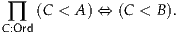 |
Then for every a : A, since A/a < A, we have A/a < B, hence there is b : B
with A/a = B/b. Define f : A → B to take each a to the corresponding b; it is
straightforward to verify that f is an isomorphism. Thus A B, hence A = B
by univalence.
B, hence A = B
by univalence.
Finally, it is easy to see that < is transitive. __
Treating Ord as an ordinal is often very convenient, but it has its pitfalls as well. For instance, consider the following lemma, where we pay attention to how universes are used.
Proof. Let B = A + 1, with the element ⋆ : 1 being greater than all
elements of A. Then B is an ordinal and it is easy to see that A B/⋆. __
This lemma illustrates a potential pitfall of the “typically ambiguous” style
of using to denote an arbitrary, unspecified universe. Consider the
following alternative proof of it.
Another putative proof of Lemma 10.3.21. Note that C < A if and only if
C = A/a for some a : A. This gives an isomorphism A Ord/A, so that
A < Ord. Thus we may take B :≡Ord. __
Ord/A, so that
A < Ord. Thus we may take B :≡Ord. __
The second proof would be valid if we had stated Lemma 10.3.21 in a typically ambiguous style. But the resulting lemma would be less useful, because the second proof would constrain the second “Ord” in the lemma statement to refer to a higher universe level than the first one. The first proof allows both universes to be the same.
Similar remarks apply to the next lemma, which could be proved in a less useful way by observing that A ≤Ord for any A : Ord.
Lemma 10.3.22. Let be a universe. For any X : and F : X → Ord,
there exists B : Ordsuch that Fx ≤ B for all x : X.
Proof. Let B be the quotient of the equivalence relation ~ on ∑(x:X) Fx defined as follows:
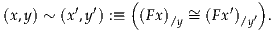
Define (x, y) < (x′, y′) if (Fx)/y < (Fx′)/y′. This clearly descends to the quotient, and can be seen to make B into an ordinal. Moreover, for each x : X the induced map Fx → B is a simulation. __
We now show the equivalence of our ordinals with the more familiar classical well-orderings.
Proof. By induction on a, we may assume that for every a′ < a and every b′ : A, we have (a′ < b′) ∨ (a′ = b′) ∨ (b′ < a′). Now by induction on b, we may assume that for every b′ < b, we have (a < b′)∨(a = b′)∨(b′ < a).
By excluded middle, either there merely exists a b′ < b such that a < b′, or there merely exists a b′ < b such that a = b′, or for every b′ < b we have b′ < a. In the first case, merely a < b by transitivity, hence a < b as it is a mere proposition. Similarly, in the second case, a < b by transport. Thus, suppose ∀(b′ : A).(b′ < b) → (b′ < a).
Now analogously, either there merely exists a′ < a such that b < a′, or there merely exists a′ < a such that a′ = b, or for every a′ < a we have a′ < b. In the first and second cases, b < a, so we may suppose ∀(a′ : A).(a′ < a) → (a′ < b). However, by extensionality, our two suppositions now imply a = b. __
Proof. We prove by induction on a : A that there is no cycle containing a. Thus, suppose by induction that for all a′ < a, there is no cycle containing a′. But in any cycle containing a, there is some element less than a and contained in the same cycle. __
In particular, a well-founded relation must be irreflexive, i.e. ¬(a < a) for all a.
Theorem 10.4.3. Assuming excluded middle, (A, <) is an ordinal if and only if every nonempty subset B ⊆ Ahas a least element.
Proof. If A is an ordinal, then by Lemma 10.3.8 every nonempty subset merely has a minimal element. But trichotomy implies that any minimal element is a least element. Moreover, least elements are unique when they exist, so merely having one is as good as having one.
Conversely, if every nonempty subset has a least element, then by
Lemma 10.3.8, A is well-founded. We also have trichotomy, since for
any a, b the subset  :≡
:≡  x = a∨x = b} merely has a least
element, which must be either a or b. This implies transitivity, since if
a < b and b < c, then either a = c or c < a would produce a cycle.
Similarly, it implies extensionality, for if ∀(c : A).(c < a) ⇔ (c < b), then
a < b implies (letting c be a) that a < a, which is a cycle, and similarly if
b < a; hence a = b. __
x = a∨x = b} merely has a least
element, which must be either a or b. This implies transitivity, since if
a < b and b < c, then either a = c or c < a would produce a cycle.
Similarly, it implies extensionality, for if ∀(c : A).(c < a) ⇔ (c < b), then
a < b implies (letting c be a) that a < a, which is a cycle, and similarly if
b < a; hence a = b. __
In classical mathematics, the characterization of Theorem 10.4.3 is taken as the definition of a well-ordering, with the ordinals being a canonical set of representatives of isomorphism classes for well-orderings. In our context, the structure identity principle means that there is no need to look for such representatives: any well-ordering is as good as any other.
We now move on to consider consequences of the axiom of choice. For any
set X, let +(X) denote the type of merely inhabited subsets of X:

Assuming excluded middle, this is equivalently the type of nonempty subsets
of X, and we have (X) ≃ (+(X)) + 1.
Of course, (i) is a standard classical version of the axiom of choice; see Exercise 10.10.
Proof. One direction is easy: suppose (ii). Since we aim to prove the mere proposition (i), we may assume A is an ordinal. But then we can define f(B) to be the least element of B.
Now suppose (i). As before, since (ii) is a mere proposition, we may assume given such an f. We extend f to a function

in the obvious way. Now for any ordinal A, we can define gA : A → X + 1 by well-founded recursion:

(regarding X as a subset of X + 1 in the obvious way).
Let A′ :≡  gA(a) ∈ X} be the preimage of X ⊆ X + 1; then
we claim the restriction gA′ : A′ → X is injective. For if a, a′ : A with
a≠a′, then by trichotomy and without loss of generality, we may assume
a′ < a. Thus gA(a′) ∈
gA(a) ∈ X} be the preimage of X ⊆ X + 1; then
we claim the restriction gA′ : A′ → X is injective. For if a, a′ : A with
a≠a′, then by trichotomy and without loss of generality, we may assume
a′ < a. Thus gA(a′) ∈  b < a}, so since f(Y) ∈ Y for all Y we
have gA(a)≠gA(a′).
b < a}, so since f(Y) ∈ Y for all Y we
have gA(a)≠gA(a′).
Moreover, A′ is an initial segment of A. For gA(a) lies in 1 if and only
if  b < a} = X, and if this holds then it also holds for any a′ > a.
Thus, A′ is itself an ordinal.
b < a} = X, and if this holds then it also holds for any a′ > a.
Thus, A′ is itself an ordinal.
Finally, since Ord is an ordinal, we can take A :≡Ord. Let X′ be the image of gOrd′ : Ord′→ X; then the inverse of gOrd′ yields an injection H : X′→Ord. By Lemma 10.3.22, there is an ordinal C such that Hx ≤ C for all x : X′. Then by Lemma 10.3.21, there is a further ordinal D such that C < D, hence Hx < D for all x : X′. Now we have
| gOrd(D) | =  X\ X\ B < D∧ (gOrd(B) ∈ X)} B < D∧ (gOrd(B) ∈ X)}
 | ||
=  X\ X\ gOrd(B) ∈ X} gOrd(B) ∈ X}
 |
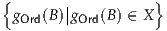
is not all of X, then gOrd(D) would lie in X but not in this subset, which would be a contradiction since D is itself a potential value for B. So this set must be all of X, and hence gOrd′ is surjective as well as injective. Thus, we can transport the ordinal structure on Ord′ to X. __
Remark 10.4.5. If we had given the wrong proof of Lemma 10.3.21 or Lemma 10.3.22, then the resulting proof of Theorem 10.4.4 would be invalid: there would be no way to consistently assign universe levels. As it is, we require propositional resizing (which follows from LEM) to ensure that X′ lives in the same universe as X (up to equivalence).
Corollary 10.4.6. Assuming the axiom of choice, the function Ord → Set (which forgets the order structure) is a surjection.
Note that Ord is a set, while Set is a 1-type. In general, there is no reason for a 1-type to admit any surjective function from a set. Even the axiom of choice does not appear to imply that every 1-type does so (although see Exercise 7.9), but it readily implies that this is so for 1-types constructed out of Set, such as the types of objects of categories of structures as in §9.8. The following corollary also applies to such categories.
Proof. Let X0 :≡ Ord, and for A, B : X0 let hom X(A, B) :≡ (A → B).
Then X is a strict category, since Ord is a set, and the above surjection
X0 →Set extends to a weak equivalence functor X →et. __
Now recall from §10.2 that we have a further surjection  0 : Set →Card,
and hence a composite surjection Ord →Card which sends each ordinal to its
cardinality.
0 : Set →Card,
and hence a composite surjection Ord →Card which sends each ordinal to its
cardinality.
Proof. There is an easy and wrong proof of this: since Ord and Card are both sets, AC implies that any surjection between them merely has a section. However, we actually have a canonical specified section: because Ord is an ordinal, every nonempty subset of it has a uniquely specified least element. Thus, we can map each cardinal to the least element in the corresponding fiber. __
It is traditional in set theory to identify cardinals with their image in Ord: the least ordinal having that cardinality.
It follows that Card also canonically admits the structure of an ordinal: in fact, one isomorphic to Ord. Specifically, we define by well-founded recursion a function ℵ : Ord →Ord, such that ℵ(A) is the least ordinal having cardinality greater than ℵ(A/a) for all a : A. Then (assuming AC) the image of ℵ is exactly the image of Card.
We can define a cumulative hierarchy V of all sets in a given universe as a
higher inductive type, in such a way that V is again a set (in a larger universe
′), equipped with a binary “membership” relation x ∈ y which satisfies the
usual laws of set theory.
Definition 10.5.1. The cumulative hierarchy V relative to a type universe
is the higher inductive type generated by the following constructors.
In set-theoretic language, set(A, f) can be understood as the set
(in the sense of classical set theory) that is the image of A under f,
i.e.  a ∈ A}. However, we will avoid this notation, since it would clash
with our notation for subtypes (but see (10.5.3) and Definition 10.5.7
below).
a ∈ A}. However, we will avoid this notation, since it would clash
with our notation for subtypes (but see (10.5.3) and Definition 10.5.7
below).
The hierarchy V is bootstrapped from the empty map rec0(V) : 0 → V ,
which gives the empty set as ∅ = set(0, rec0(V)). Then the singleton {∅}
enters V through 1 → V , defined as ⋆ ∅, and so on. The type V lives in the
same universe as the base universe .
∅, and so on. The type V lives in the
same universe as the base universe .
The second constructor of V has a form unlike any we have seen before: it involves not only paths in V (which in §6.9 we claimed were slightly fishy) but truncations of sums of them. It certainly does not fit the general scheme described in §6.13, and thus it may not be obvious what its induction principle should be. Fortunately, like our first definition of the 0-truncation in §6.9, it can be re-expressed using auxiliary higher inductive types. We leave it to the reader to work out the details (see Exercise 10.11).
At the end of the day, the induction principle for V (written in pattern matching language) says that given P : V →Set, in order to construct h : ∏(x:V) P(x), it suffices to give the following.
The second clause checks that the map being defined must respect the paths introduced in (10.5.2). As usual when we state higher induction principles using pattern matching, it may seem tautologous, but is not. The point is that “h(f(a))” is essentially a formal symbol which we cannot peek inside of, which h(set(A, f)) must be defined in terms of. Thus, in the second clause, we assume equality of these formal symbols when appropriate, and verify that the elements resulting from the construction of the first clause are also equal. Of course, if P is a family of mere propositions, then the second clause is automatic.
Observe that, by induction, for each v : V there merely exist A : and
f : A → V such that v = set(A, f). Thus, it is reasonable to try to define the
membership relation x ∈ v on V by setting:
 |
To see that the definition is valid, we must use the recursion principle of V . Thus, suppose we have a path set(A, f) = set(B, g) constructed through (10.5.2). If x ∈set(A, f) then there merely is a : A such that x = f(a), but by (10.5.2) there merely is b : B such that f(a) = g(b), hence x = g(b) and x ∈set(B, f). The converse is symmetric.
The subset relation x ⊆ y is defined on V as usual by
 |
A class may be taken to be a mere predicate on V . We can say that a class C : V →Prop is a V-set if there merely exists v ∈ V such that
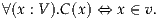 |
We may also use the conventional notation for classes, which matches our standard notation for subtypes:
 | (10.5.3) |
A class C : V →Prop will be called -small if all of its values C(x) lie in ,
specifically C : V →Prop. Since V lives in the same universe ′ as does the
base universe from which it is built, the same is true for the identity types
v = Vw for any v, w : V . To obtain a well-behaved theory in the absence of
propositional resizing, therefore, it will be convenient to have a -small
“resizing” of the identity relation, which we can define by induction as
follows.
Definition 10.5.4. Define the bisimulation relation
 |
by double induction over V , where for set(A, f) and set(B, g) we let:

To verify that the definition is correct, we just need to check that it respects
paths set(A, f) = set(B, g) constructed through (10.5.2), but this is
obvious, and that Prop is a set, which it is. Note that u ~ v is in Prop by
construction.
Proof. An easy induction shows that ~ is reflexive, so by transport we have (u = Vv) → (u ~ v). Thus, it remains to show that (u ~ v) → (u = Vv). By induction on u and v, we may assume they are set(A, f) and set(B, g) respectively. Then by definition, set(A, f) ~ set(B, g) implies (∀(a : A).∃(b : B).f(a) ~ g(b)) and conversely. But the inductive hypothesis then tells us that (∀(a : A).∃(b : B).f(a) = g(b)) and conversely. So by the path-constructor for V we have set(A, f) = Vset(B, g). __
Now we can use the resized identity relation to get the following useful principle.
Lemma 10.5.6. For every u : V there is a given Au : and monic mu :
Au ↣ V such that u = set(Au, mu).
Proof. Take any presentation u = set(A, f) and factor f : A → V as a surjection followed by an injection:
 |
Clearly u = set(Au, mu) if only Au is still in , which holds if the kernel of
eu : A ↠ Au is in . But the kernel of eu : A ↠ Au is the pullback
along f : A → V of the identity on V , which we just showed to be
-small, up to equivalence. Now, this construction of the pair (Au, mu)
with mu : Au ↣ V and u = set(Au, mu) from u : V is unique up to
equivalence over V , and hence up to identity by univalence. Thus by the
principle of unique choice (3.9.2) there is a map c : V → ∑(A:) (A → V)
such that c(u) = (Au, mu), with mu : Au ↣ V and u = set(c(u)), as
claimed. __
Definition 10.5.7. For u : V , the just constructed monic presentation mu : Au ↣ V such that u = set(Au, mu) may be called the type of members of u and denoted mu : [u] ↣ V , or even [u] ↣ V . We can think of [u] as the “subclass of V consisting of members of u”.
Theorem 10.5.8. The following hold for (V , ∈):
 |
 x = u∨x = v}is a
V-set.
x = u∨x = v}is a
V-set.
 ∃(u : V).x ∈ u ∈ v}is a
V-set.
∃(u : V).x ∈ u ∈ v}is a
V-set.
 x : u → v}is a
V-set.1
x : u → v}is a
V-set.1
 |
is a V-set.
-small C : V →Prop, the class
 |
is a V-set.
Sketch of proof.
-small,
and we have ∪v :≡set(Ã, λx.mf(pr1(x))(pr2(x))).
![r : ([u] → [v]) -→ V](hott-html3925x.png)
with “r(f) =  x : [u]}”, but in order for this to make
sense we must first define the ordered pair (x, y), and then we take
the map r′ : x
x : [u]}”, but in order for this to make
sense we must first define the ordered pair (x, y), and then we take
the map r′ : x (x, f(x)), and then we can put r(f) :≡set([u], r′).
But the ordered pair can be defined in terms of unordered pairing
as usual.
(x, f(x)), and then we can put r(f) :≡set([u], r′).
But the ordered pair can be defined in terms of unordered pairing
as usual.
 |
is a V -set. We need to show that any -small C : V →Prop is
separable. Indeed, given a = set(A, f), let A′ = ∃(x : A).C(fx), and take
f′ = f ∘i, where i : A′→ A is the obvious inclusion. Then we
can take a′ = set(A′, f′) and we have x ∈ a∧C(x) ⇔ x ∈ a′ as
claimed. We needed the assumption that C lands in in order for
A′ = ∃(x : A).C(fx) to be in . __
It is also convenient to have a strictly syntactic criterion of separability, so that one can read off from the expression for a class that it produces a V -set. One such familiar condition is being “Δ0”, which means that the expression is built up from equality x = Vy and membership x ∈ y, using only mere-propositional connectives ¬, ∧, ∨, ⇒ and quantifiers ∀, ∃ over particular sets, i.e. of the form ∃(x ∈ a) and ∀(y ∈ b) (these are called bounded quantifiers).
Proof. Recall that we have a -small resizing x ~ y of identity x = y. Since
x ∈ y is defined in terms of x = y, we also have a -small resizing of
membership
 |
Now, let Φ be a Δ0 expression for C, so that as classes Φ = C (strictly
speaking, we should distinguish expressions from their meanings, but we will
blur the difference). Let  be the result of replacing all occurrences of = and ∈
by their resized equivalents ~ and
be the result of replacing all occurrences of = and ∈
by their resized equivalents ~ and  . Clearly then
  also expresses C, in the
sense that for all x : V ,
also expresses C, in the
sense that for all x : V ,  (x) ⇔ C(x), and hence
  = C by univalence. It now
suffices to show that
= C by univalence. It now
suffices to show that  is -small, for then it will be separable by the
theorem.
is -small, for then it will be separable by the
theorem.
We show that  is -small by induction on the construction of the
expression. The base cases are x ~ y and x
is -small by induction on the construction of the
expression. The base cases are x ~ y and x  y, which have already been
resized into . It is also clear that is closed under the mere-propositional
operations (and (-1)-truncation), so it just remains to check the bounded
quantifiers ∃(x ∈ a) and ∀(y ∈ b). By definition,
y, which have already been
resized into . It is also clear that is closed under the mere-propositional
operations (and (-1)-truncation), so it just remains to check the bounded
quantifiers ∃(x ∈ a) and ∀(y ∈ b). By definition,
| ∃(x ∈ a)P(x) | :≡ ∑
x:V (x ∑
x:V (x  a∧P(x)) a∧P(x)) , , | ||
| ∀(y ∈ b)P(x) | :≡ ∏
x:V (x  a → P(x)). a → P(x)). |
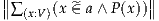 . Although the body (x
  a∧P(x)) is
-small since P(x) is so by the inductive hypothesis, the quantification over V
need not stay inside . However, in the present case we can replace this with
a quantification over the type [a] ↣ V of members of a, and easily show
that
a∧P(x)) is
-small since P(x) is so by the inductive hypothesis, the quantification over V
need not stay inside . However, in the present case we can replace this with
a quantification over the type [a] ↣ V of members of a, and easily show
that
![(x ^∈ a ∧ P(x)) = P(x).
∑x:V ∑x:[a]](hott-html3950x.png) |
The right-hand side does remain in , since both [a] and P(x)
are in . The case of ∏(x:V) (x  a → P(x)) is analogous, using
∏
(x:V) (x
a → P(x)) is analogous, using
∏
(x:V) (x  a → P(x)) = ∏(x:[a]) P(x). __
We have shown that in type theory with a universe , the cumulative
hierarchy V is a model of a “constructive set theory” with many of the
standard axioms. However, as far as we know, it lacks the strong collection and
subset collection axioms which are included in Constructive Zermelo–Fraenkel
Set Theory [Acz78]. In the usual interpretation of this set theory into type
theory, these two axioms are consequences of the setoid-like definition of
equality; while in other constructed models of set theory, strong collection
may hold for other reasons. We do not know whether either of these
axioms holds in our model (V , ∈), but it seems unlikely. Since V is a
higher inductive type inside the system, rather than being an external
construction, it is not surprising that it differs in some ways from prior
interpretations.
Finally, consider the result of adding the axiom of choice for sets
to our type theory, in the form AC from §10.1.5 above. This has the
consequence that LEM then also holds, by Theorem 10.1.14, and so Set is a
topos with subobject classifier 2, by Theorem 10.1.12. In this case,
we have Prop = 2 : , and so all classes are separable. Thus we have
shown:
Lemma 10.5.10. In type theory with AC, the law of (full) separation holds for V: given any class C : V →Prop and a : V, the class a∩C is a V-set.
Theorem 10.5.11. In type theory with AC and a universe , the cumulative
hierarchy V is a model of Zermelo–Fraenkel set theory with choice, ZFC.
Proof. We have all the axioms listed in Theorem 10.5.8, plus full
separation, so we just need to show that there are power sets (a) : V
for all a : V . But since we have LEM these are simply function types
(a) = (a →2). Thus V is a model of Zermelo–Fraenkel set theory ZF.
We leave the verification of the set-theoretic axiom of choice from AC as
an easy exercise. __
The basic properties one expects of the category of sets date back to the early days of elementary topos theory. The Elementary theory of the category of sets referred to in §10.1.5 was introduced by Lawvere in [Law05], as a category-theoretic axiomatization of set theory. The notion of ΠW-pretopos, regarded as a predicative version of an elementary topos, was introduced in [MP02]; see also [Pal09].
The treatment of the category of sets in §10.1 roughly follows that
in [RS13]. The fact that epimorphisms are surjective (Lemma 10.1.4) is
well known in classical mathematics, but is not as trivial as it may
seem to prove predicatively. The proof in [MRR88] uses the power set
operation (which is impredicative), although it can also be seen as a
predicative proof of the weaker statement that a map in a universe
i is surjective if it is an epimorphism in the next universe i+1. A
predicative proof for setoids was given by Wilander [Wil10]. Our proof
is similar to Wilander’s, but avoids setoids by using pushouts and
univalence.
The implication in Theorem 10.1.14 from AC to LEM is an adaptation to homotopy type theory of a theorem from topos theory due to Diaconescu [Dia75]; it was posed as a problem already by Bishop [Bis67, Problem 2].
For the intuitionistic theory of ordinal numbers, see [Tay96] and also [JM95]. Definitions of well-foundedness in type theory by an induction principle, including the inductive predicate of accessibility, were studied in [Hue80, Pau86, Nor88], although the idea dates back to Gentzen’s proof of the consistency of arithmetic [Gen36].
The idea of algebraic set theory, which informs our development in §10.5 of the cumulative hierarchy, is due to [JM95], but it derives from earlier work by [Acz78].
Exercise 10.1. Following the pattern of et, we would like to make a
category  ype of all types and maps between them (in a given universe
). In order for this to be a category in the sense of §9.1, however, we
must first declare hom(X, Y) :≡
ype of all types and maps between them (in a given universe
). In order for this to be a category in the sense of §9.1, however, we
must first declare hom(X, Y) :≡ 0, with composition defined
by induction on truncation from ordinary composition (Y → Z) →
(X → Y) → (X → Z). This was defined as the homotopy precategory
of types in Example 9.1.18. It is still not a category, however, but only
a precategory (its type of objects is not even a 0-type). It becomes a
category by Rezk completion (see Example 9.9.7), and its type of objects
can be identified with
0, with composition defined
by induction on truncation from ordinary composition (Y → Z) →
(X → Y) → (X → Z). This was defined as the homotopy precategory
of types in Example 9.1.18. It is still not a category, however, but only
a precategory (its type of objects is not even a 0-type). It becomes a
category by Rezk completion (see Example 9.9.7), and its type of objects
can be identified with  1 by Exercise 9.9. Show that the resulting
category ype, unlike et, is not a pretopos.
1 by Exercise 9.9. Show that the resulting
category ype, unlike et, is not a pretopos.
Exercise 10.2. Show that if every surjection has a section in the category
et, then the axiom of choice holds.
Exercise 10.3. Show that with LEM, the category et is well-pointed, in
the sense that the following statement holds: for any f, g : A → B, if
f≠g then there is a function a : 1 → A such that f(a)≠g(a). Show that
the slice category et/2 consisting of functions A →2 and commutative
triangles does not have this property. (Hint: the terminal object in et/2
is the identity function 2 →2, so in this category, there are objects X that
have no elements 1 → X.)
Exercise 10.4. Prove that if (A, < A) and (B, < B) are well-founded, extensional, or ordinals, then so is A + B, with < defined by
| (a < a′) | :≡ (a < Aa′) | for | a, a′ : A | ||||
| (b < b′) | :≡ (b < Bb′) | for | b, b′ : B | ||||
| (a < b) | :≡1 | for | (a : A), (b : B) | ||||
| (b < a) | :≡0 | for | (a : A), (b : B). |
Exercise 10.5. Prove that if (A, < A) and (B, < B) are well-founded, extensional, or ordinals, then so is A×B, with < defined by

Exercise 10.6. Define the usual algebraic operations on ordinals, and prove that they satisfy the usual properties.
Exercise 10.7. Note that 2 is an ordinal, under the obvious relation < such that 02 < 12 only.
Exercise 10.8. Recall that we denote N by ω when regarding it as an ordinal; thus we have also the ordinal ω + 1. On the other hand, let us define

where ≤ denotes the obvious partial order on 2, with 02 ≤ 12.
Exercise 10.9. Show that if (A, <) is well-founded and extensional and
A : , then there is a simulation A → V , where (V , ∈) is the cumulative
hierarchy from §10.5 built from the universe .
Exercise 10.10. Show that Theorem 10.4.4(i) is equivalent to the axiom of choice (3.8.1).
Exercise 10.11. Given types A and B, define a bitotal relation to be R : A → B →Prop such that

For such A, B, R, let A⊔RB be the higher inductive type generated by
Show that the cumulative hierarchy V can be defined by the following more straightforward list of constructors, and that the resulting induction principle is the one given in §10.5.
Exercise 10.12. In Constructive Zermelo–Fraenkel Set Theory, the axiom of strong collection has the form:
![∀(x ∈ v).∃ (y).R(x,y) ⇒
∃(w).[(∀(x ∈ v).∃(y ∈ w).R(x,y))∧(∀(y ∈ w).∃ (x ∈ v).R(x,y))]](hott-html3972x.png) |
Exercise 10.13. Verify that, if we assume AC, then the cumulative hierarchy V satisfies the usual set-theoretic axiom of choice, which may be stated in the form:

Any foundation of mathematics worthy of its name must eventually address the construction of real numbers as understood by mathematical analysis, namely as a complete archimedean ordered field. There are two notions of completeness. The one by Cauchy requires that the reals be closed under limits of Cauchy sequences, while the stronger one by Dedekind requires closure under Dedekind cuts. These lead to two ways of constructing reals, which we study in §11.2 and §11.3, respectively. In Theorems 11.2.14 and 11.3.50 we characterize the two constructions in terms of universal properties: the Dedekind reals are the final archimedean ordered field, and the Cauchy reals the initial Cauchy complete archimedean ordered field.
In traditional constructive mathematics, real numbers always seem to require certain compromises. For example, the Dedekind reals work better with power sets or some other form of impredicativity, while Cauchy reals work well in the presence of countable choice. However, we give a new construction of the Cauchy reals as a higher inductive-inductive type that seems to be a third possibility, which requires neither power sets nor countable choice.
In §11.4 we compare the two constructions of reals. The Cauchy reals are included in the Dedekind reals. They coincide if excluded middle or countable choice holds, but in general the inclusion might be proper.
In §11.5 we consider three notions of compactness of the closed interval [0, 1]. We first show that [0, 1] is metrically compact in the sense that it is complete and totally bounded, and that uniformly continuous maps on metrically compact spaces behave as expected. In contrast, the Bolzano–Weierstraß property that every sequence has a convergent subsequence implies the limited principle of omniscience, which is an instance of excluded middle. Finally, we discuss Heine-Borel compactness. A naive formulation of the finite subcover property does not work, but a proof relevant notion of inductive covers does. This section is basically standard constructive analysis.
The development of real numbers and analysis in homotopy type theory can be easily made compatible with classical mathematics. By assuming excluded middle and the axiom of choice we get standard classical analysis: the Dedekind and Cauchy reals coincide, foundational questions about the impredicative nature of the Dedekind reals disappear, and the interval is as compact as it could be.
We close the chapter by constructing Conway’s surreals as a higher inductive-inductive type in §11.6; the construction is more natural in univalent type theory than in classical set theory.
In addition to the basic theory of Chapters 2 and 3, as noted above we use “higher inductive-inductive types” for the Cauchy reals and the surreals: these combine the ideas of Chapter 6 with the notion of inductive-inductive type mentioned in §5.7. We will also frequently use the traditional logical notation described in §3.7, and the fact (proven in §10.1) that our “sets” behave the way we would expect.
Note that the total space of the universal cover of the circle, which in §8.1.5 played a role similar to “the real numbers” in classical algebraic topology, is not the type of reals we are looking for. That type is contractible, and thus equivalent to the singleton type, so it cannot be equipped with a non-trivial algebraic structure.
We first construct the rational numbers Q, as the reals can then be seen as a completion of Q. An expert will point out that Q could be replaced by any approximate field, i.e., a subring of Q in which arbitrarily precise approximate inverses exist. An example is the ring of dyadic rationals, which are those of the form n/2k. If we were implementing constructive mathematics on a computer, an approximate field would be more suitable, but we leave such finesse for those who care about the digits of π.
We constructed the integers Z in §6.10 as a quotient of N ×N, and observed that this quotient is generated by an idempotent. In §6.11 we saw that Z is the free group on 1; we could similarly show that it is the free commutative ring on 0. The field of rationals Q is constructed along the same lines as well, namely as the quotient

where

In other words, a pair (u, a) represents the rational number u/(1 + a). There can be no division by zero because we cunningly added one to the denominator a. Here too we have a canonical choice of representatives, namely fractions in lowest terms. Thus we may apply Lemma 6.10.8 to obtain a set Q, which again has a decidable equality.
We do not bother to write down the arithmetical operations on Q as we trust our readers know how to compute with fractions even in the case when one is added to the denominator. Let us just record the conclusion that there is an entirely unproblematic construction of the ordered field of rational numbers Q, with a decidable equality and decidable order. It can also be characterized as the initial ordered field.
Let Q+ =  q > 0} be the type of positive rational numbers.
Let us first recall the basic idea of Dedekind’s construction. We use two-sided Dedekind cuts, as opposed to an often used one-sided version, because the symmetry makes constructions more elegant, and it works constructively as well as classically. A Dedekind cut consists of a pair (L, U) of subsets L, U ⊆Q, called the lower and upper cut respectively, which are:
Reading the roundedness condition from left to right tells us that cuts are open, and from right to left that they are lower, respectively upper, sets. The locatedness condition states that there is no large gap between L and U. Because cuts are always open, they never include the “point in between”, even when it is rational. A typical Dedekind cut looks like this:
L U
We might naively translate the informal definition into type theory by saying that
a cut is a pair of maps L, U : Q →Prop. But we saw in §3.5 that Prop is an
ambiguous notation for Propi where i is a universe. Once we use a
particular i to define cuts, the type of reals will reside in the next universe
i+1, a property of reals two levels higher in i+2, a property of subsets of
reals in i+3, etc. In principle we should be able to keep track of the universe
levels, especially with the help of a proof assistant, but doing so here would
just burden us with bureaucracy that we prefer to avoid. We shall therefore
make a simplifying assumption that a single type of propositions Ω is
sufficient for all our purposes.
In fact, the construction of the Dedekind reals is quite resilient to logical manipulations. There are several ways in which we can make sense of using a single type Ω:
i’s to the lowest level, which
we call Ω.
In all of the above cases Ω is a set. Without further ado, we translate the informal definition into type theory. Throughout this chapter, we use the logical notation from Definition 3.7.1.
Definition 11.2.1. A Dedekind cut is a pair (L, U) of mere predicates L : Q → Ω and U : Q → Ω which is:
| L(q) | ⇔∃(r : Q).(q < r) ∧L(r) and | ||
| U(r) | ⇔∃(q : Q).(q < r) ∧U(q), |
We let isCut(L, U) denote the conjunction of these conditions. The type of Dedekind reals is
 |
It is apparent that isCut(L, U) is a mere proposition, and since Q → Ω is a set the Dedekind reals form a set too. See Exercises 11.2 to 11.4 for variants of Dedekind cuts which lead to extended reals, lower and upper reals, and the interval domain.
There is an embedding Q →Rd which associates with each rational q : Q the cut (Lq, Uq) where
 |
We shall simply write q for the cut (Lq, Uq) associated with a rational number.
The construction of the algebraic and order-theoretic structure of Dedekind reals proceeds as usual in intuitionistic logic. Rather than dwelling on details we point out the differences between the classical and intuitionistic setup. Writing Lx and Ux for the lower and upper cut of a real number x : Rd, we define addition as
| Lx+y(q) | :≡∃(r, s : Q).Lx(r) ∧Ly(s) ∧q = r + s, | ||
| Ux+y(q) | :≡∃(r, s : Q).Ux(r) ∧Uy(s) ∧q = r + s, |
| L-x(q) | :≡∃(r : Q).Ux(r) ∧q = -r, | ||
| U-x(q) | :≡∃(r : Q).Lx(r) ∧q = -r. |
| Lx⋅y(q) | :≡∃(a, b, c, d : Q).Lx(a) ∧Ux(b) ∧Ly(c) ∧Uy(d) ∧ q < min(a⋅c, a⋅d, b⋅c, b⋅d), | ||
| Ux⋅y(q) | :≡∃(a, b, c, d : Q).Lx(a) ∧Ux(b) ∧Ly(c) ∧Uy(d) ∧ max(a⋅c, a⋅d, b⋅c, b⋅d) < q. |
![[a,b]⋅[c,d] = [m in(ac,ad,bc,bd),m ax(ac,ad,bc,bd)].](hott-html4005x.png) |
For instance, the formula for the lower cut can be read as saying that q < x⋅y when there are intervals [a, b] and [c, d] containing x and y, respectively, such that q is to the left of [a, b] ⋅ [c, d]. It is generally useful to think of an interval [a, b] such that Lx(a) and Ux(b) as an approximation of x, see Exercise 11.4.
We now have a commutative ring with unit (Rd, 0, 1, +, -, ⋅). To treat multiplicative inverses, we must first introduce order. Define ≤ and < as
| (x ≤ y) | :≡ ∀(q : Q).Lx(q) ⇒ Ly(q), | ||
| (x < y) | :≡ ∃(q : Q).Ux(q) ∧Ly(q). |
Proof. If Lx(q) then by roundedness there merely is r > q such that Lx(r), and since Uq(r) it follows that q < x. Conversely, if q < x then there is r : Q such that Uq(r) and Lx(r), hence Lx(q) because Lx is a lower set. The other half of the proof is symmetric. __
The relation ≤ is a partial order, and < is transitive and irreflexive. Linearity
 |
is valid if we assume excluded middle, but without it we get weak linearity
 | (11.2.3) |
At first sight it might not be clear what (11.2.3) has to do with linear order. But if we take x ≡ u-ϵ and y ≡ u + ϵ for ϵ > 0, then we get
 |
This is linearity “up to a small numerical error”, i.e., since it is unreasonable to expect that we can actually compute with infinite precision, we should not be surprised that we can decide < only up to whatever finite precision we have computed.
To see that (11.2.3) holds, suppose x < y. Then there merely exists q : Q such that Ux(q) and Ly(q). By roundedness there merely exist r, s : Q such that r < q < s, Ux(r) and Ly(s). Then, by locatedness Lz(r) or Uz(s). In the first case we get x < z and in the second z < y.
Classically, multiplicative inverses exist for all numbers which are different from zero. However, without excluded middle, a stronger condition is required. Say that x, y : Rd are apart from each other, written x # y, when (x < y) ∨ (y < x):
 |
If x # y, then ¬(x = y). The converse is true if we assume excluded middle, but is not provable constructively. Indeed, if ¬(x = y) implies x # y, then a little bit of excluded middle follows; see Exercise 11.10.
Remark 11.2.5. We observe that a real is invertible if, and only if, it is merely invertible. Indeed, the same is true in any ring, since a ring is a set, and multiplicative inverses are unique if they exist. See the discussion following Corollary 3.9.2.
Proof. Suppose x⋅y = 1. Then there merely exist a, b, c, d : Q such that a < x < b, c < y < d and 0 < min(ac, ad, bc, bd). From 0 < ac and 0 < bc it follows that a, b, and c are either all positive or all negative. Hence either 0 < a < x or x < b < 0, so that x # 0.
Conversely, if x # 0 then
| Lx-1(q) | :≡∃(r : Q).Ux(r) ∧ ((0 < r∧qr < 1) ∨ (r < 0 ∧ 1 < qr)) | ||
| Ux-1(q) | :≡∃(r : Q).Lx(r) ∧ ((0 < r∧qr > 1) ∨ (r < 0 ∧ 1 > qr)) |
The archimedean principle can be stated in several ways. We find it most illuminating in the form which says that Q is dense in Rd.
Theorem 11.2.6 (Archimedean principle for Rd). For all x, y : Rd if x < ythen there merely exists q : Q such that x < q < y.
Proof. By definition of <. __
Before tackling completeness of Dedekind reals, let us state precisely what algebraic structure they possess. In the following definition we are not aiming at a minimal axiomatization, but rather at a useful amount of structure and properties.
Definition 11.2.7. An ordered field is a set F together with constants 0, 1, operations +, -, ⋅, min, max, and mere relations ≤, <, # such that:
| x ≤ y | ⇔¬(y < x), | x < y ≤ z | ⇒ x < z, | ||||
| x # y | ⇔ (x < y) ∨ (y < x), | x ≤ y < z | ⇒ x < z, | ||||
| x ≤ y | ⇔ x + z ≤ y + z, | x ≤ y∧ 0 ≤ z | ⇒ xz ≤ yz, | ||||
| x < y | ⇔ x + z < y + z, | 0 < z ⇒ (x < y | ⇔ xz < yz), | ||||
| 0 < x + y | ⇒ 0 < x∨ 0 < y, | 0 | < 1. |
Every such field has a canonical embedding Q → F. An ordered field is archimedean when for all x, y : F, if x < y then there merely exists q : Q such that x < q < y.
Proof. We omit the proof in the hope that what we have demonstrated so far makes the theorem plausible. __
Recall that x : N →Q is a Cauchy sequence when it satisfies
 | (11.2.9) |
Note that we did not truncate the inner existential because we actually want to
compute rates of convergence—an approximation without an error estimate
carries little useful information. By Theorem 2.15.7, (11.2.9) yields a function
M : Q+ →N, called the modulus of convergence, such that m, k ≥ M(ϵ) implies
|xm-xk| < ϵ. From this we get |xM(δ/2) -xM(ϵ/2)| < δ + ϵ for all ϵ : Q+. In
fact, the map (ϵ xM(ϵ/2)) : Q+ →Q carries the same information
about the limit as the original Cauchy condition (11.2.9). We shall
work with these approximation functions rather than with Cauchy
sequences.
xM(ϵ/2)) : Q+ →Q carries the same information
about the limit as the original Cauchy condition (11.2.9). We shall
work with these approximation functions rather than with Cauchy
sequences.
Definition 11.2.10. A Cauchy approximation is a map x : Q+ →Rd which satisfies
 | (11.2.11) |
The limit of a Cauchy approximation x : Q+ →Rd is a number ℓ : Rd such that
 |
Proof. Note that we are showing existence, not mere existence, of the limit. Given a Cauchy approximation x : Q+ →Rd, define
| Ly(q) | :≡∃(ϵ, θ : Q+).Lxϵ(q + ϵ + θ), | ||
| Uy(q) | :≡∃(ϵ, θ : Q+).Uxϵ(q-ϵ-θ). |
To show that y is the limit of x, consider any ϵ, θ : Q+. Because Q is dense in Rd there merely exist q, r : Q such that

 |
and in the second
 |
In either case it follows that |y-xϵ| < ϵ + θ. __
For sake of completeness we record the classic formulation as well.
Corollary 11.2.13. Suppose x : N →Rd satisfies the Cauchy condition (11.2.9). Then there exists y : Rd such that
 |
Proof. By Theorem 2.15.7 there is M : Q+ →N such that (ϵ) :≡ xM(ϵ/2) is a Cauchy approximation. Let y be its limit, which exists by Theorem 11.2.12. Given any ϵ : Q+, let n :≡ M(ϵ/4) and observe that, for any m ≥ n,

We obtained Rd as the type of Dedekind cuts on Q. But we could have instead started with any archimedean ordered field F and constructed Dedekind cuts on F. These would again form an archimedean ordered field , the Dedekind completion of F, with F contained as a subfield. What happens if we apply this construction to Rd, do we get even more real numbers? The answer is negative. In fact, we shall prove a stronger result: Rd is final.
Say that an ordered field F is admissible for Ω when the strict order < on F is a map < : F → F → Ω.
Proof. Let F be an archimedean ordered field. For every x : F define L, U : Q → Ω by
 |
(We have just used the assumption that F is admissible for Ω.) Then (Lx, Ux) is a Dedekind cut. Indeed, the cuts are inhabited and rounded because F is archimedean and < is transitive, disjoint because < is irreflexive, and located because < is a weak linear order. Let e : F →Rd be the map e(x) :≡ (Lx, Ux).
We claim that e is a field embedding which preserves and reflects the order. First of all, notice that e(q) = q for a rational number q. Next we have the equivalences, for all x, y : F,

 |
The implication from right to left is obvious. For the other direction, if q < x + y then there merely exists r : Q such that q-y < r < x, and by taking s :≡ q-r we get the desired r and s. We leave preservation of multiplication by e as an exercise. __
To establish that the Dedekind cuts on Rd do not give us anything new, we need just one more lemma.
Proof. Let be the Dedekind completion of F. The strict order on is defined by
 |
Since U(q) and L′(q) are elements of Ω, the lemma holds as long as Ω is closed under conjunctions and countable existentials, which we assumed from the outset. __
Corollary 11.2.16. The Dedekind reals are Dedekind complete: for every real-valued Dedekind cut (L, U) there is a unique x : Rd such that L(y) = (y < x) and U(y) = (x < y) for all y : Rd.
Proof. By Lemma 11.2.15 the Dedekind completion d of Rd is admissible for Ω, so by Theorem 11.2.14 we have an embedding d → Rd, as well as an embedding Rd → d. But these embeddings must be isomorphisms, because their compositions are order-preserving field homomorphisms which fix the dense subfield Q, which means that they are the identity. The corollary now follows immediately from the fact that d →Rd is an isomorphism. __
The Cauchy reals are, by intent, the completion of Q under limits of Cauchy
sequences. In the classical construction of the Cauchy reals, we consider the
set of all Cauchy sequences in Q and then form a suitable quotient /≈.
Then, to show that /≈ is Cauchy complete, we consider a Cauchy sequence
x : N →/≈, lift it to a sequence of sequences : N →, and construct the
limit of x using . However, the lifting of x to uses the axiom of
countable choice (the instance of (3.8.1) where X = N) or the law of
excluded middle, which we may wish to avoid. Every construction of reals
whose last step is a quotient suffers from this deficiency. There are three
common ways out of the conundrum in constructive mathematics:
, ≈), i.e., the type of
Cauchy sequences with a coincidence relation attached to it
by administrative decree. A sequence of reals then simply is a
sequence of Cauchy sequences representing them.
Using higher inductive types, however, there is a fourth solution, which we believe to be preferable to any of the above, and interesting even to a classical mathematician. The idea is that the Cauchy real numbers should be the free complete metric space generated by Q. In general, the construction of a free gadget of any sort requires applying the gadget operations repeatedly many times to the generators. For instance, the elements of the free group on a set X are not just binary products and inverses of elements of X, but words obtained by iterating the product and inverse constructions. Thus, we might naturally expect the same to be true for Cauchy completion, with the relevant “operation” being “take the limit of a Cauchy sequence”. (In this case, the iteration would have to take place transfinitely, since even after infinitely many steps there will be new Cauchy sequences to take the limit of.)
The argument referred to above shows that if excluded middle or countable choice hold, then Cauchy completion is very special: when building the completion of a space, it suffices to stop applying the operation after one step. This may be regarded as analogous to the fact that free monoids and free groups can be given explicit descriptions in terms of (reduced) words. However, we saw in §6.11 that higher inductive types allow us to construct free gadgets directly, whether or not there is also an explicit description available. In this section we show that the same is true for the Cauchy reals (a similar technique would construct the Cauchy completion of any metric space; see Exercise 11.9). Specifically, higher inductive types allow us to simultaneously add limits of Cauchy sequences and quotient by the coincidence relation, so that we can avoid the problem of lifting a sequence of reals to a sequence of representatives.
The construction of the Cauchy reals Rc as a higher inductive type is a bit more subtle than that of the free algebraic structures considered in §6.11. We intend to include a “take the limit” constructor whose input is a Cauchy sequence of reals, but the notion of “Cauchy sequence of reals” depends on having some way to measure the “distance” between real numbers. In general, of course, the distance between two real numbers will be another real number, leading to a potentially problematic circularity.
However, what we actually need for the notion of Cauchy sequence of reals is not the general notion of “distance”, but a way to say that “the distance between two real numbers is less than ϵ” for any ϵ : Q+. This can be represented by a family of binary relations, which we will denote ~ϵ : Rc →Rc →Prop. The intended meaning of x ~ϵ y is |x-y| < ϵ, but since we do not have notions of subtraction, absolute value, or inequality available yet (we are only just defining Rc, after all), we will have to define these relations ~ϵ at the same time as we define Rc itself. And since ~ϵ is a type family indexed by two copies of Rc, we cannot do this with an ordinary mutual (higher) inductive definition; instead we have to use a higher inductive-inductive definition.
Recall from §5.7 that the ordinary notion of inductive-inductive definition allows us to define a type and a type family indexed by it by simultaneous induction. Of course, the “higher” version of this allows both the type and the family to have path constructors as well as point constructors. We will not attempt to formulate any general theory of higher inductive-inductive definitions, but hopefully the description we will give of Rc and ~ϵ will make the idea transparent.
Remark 11.3.1. We might also consider a higher inductive-recursive definition, in which ~ϵ is defined using the recursion principle of Rc, simultaneously with the inductive definition of Rc. We choose the inductive-inductive route instead for two reasons. Firstly, higher inductive-recursive definitions seem to be more difficult to justify in homotopical semantics. Secondly, and more importantly, the inductive-inductive definition yields a more powerful induction principle, which we will need in order to develop even the basic theory of Cauchy reals.
Finally, as we did for the discussion of Cauchy completeness of the Dedekind reals in §11.2.2, we will work with Cauchy approximations (Definition 11.2.10) instead of Cauchy sequences. Of course, our Cauchy approximations will now consist of Cauchy reals, rather than Dedekind reals or rational numbers.
Definition 11.3.2. Let Rc and the relation ~ : Q+ ×Rc ×Rc → be the
following higher inductive-inductive type family. The type Rc of Cauchy
reals is generated by the following constructors:
 | (11.3.3) |
there is a point lim(x) : Rc. We call x a Cauchy approximation.
 | (11.3.4) |
then there is a path eqRc(u, v) : u =Rc v.
Simultaneously, the type family ~ : Rc →Rc →Q+ → is generated by the
following constructors. Here q and r denote rational numbers; δ, ϵ, and η
denote positive rationals; u and v denote Cauchy reals; and x and y denote
Cauchy approximations:
The first constructor of Rc says that any rational number can be regarded as a real number. The second says that from any Cauchy approximation to a real number, we can obtain a new real number called its “limit”. And the third expresses the idea that if two Cauchy approximations coincide, then their limits are equal.
The first four constructors of ~ specify when two rational numbers are close, when a rational is close to a limit, and when two limits are close. In the case of two rational numbers, this is just the usual notion of ϵ-closeness for rational numbers, whereas the other cases can be derived by noting that each approximant xδ is supposed to be within δ of the limit lim(x).
We remind ourselves of proof-relevance: a real number obtained from lim is represented not just by a Cauchy approximation x, but also a proof p of (11.3.3), so we should technically have written lim(x, p) instead of just lim(x). A similar observation also applies to eqRc and (11.3.4), but we shall write just eqRc : u = v instead of eqRc(u, v, p) : u = v. These abuses of notation are mitigated by the fact that we are omitting mere propositions and information that is readily guessed. Likewise, the last constructor of ~ϵ justifies our leaving the other four nameless.
We are immediately able to populate Rc with many real numbers. For
suppose x : N →Q is a traditional Cauchy sequence of rational numbers, and
let M : Q+ →N be its modulus of convergence. Then rat ∘x∘M : Q+ →Rc
is a Cauchy approximation, using the first constructor of ~ to produce the
necessary witness. Thus, lim(rat ∘x∘m) is a real number. Various famous
real numbers  , π, e, … are all limits of such Cauchy sequences of
rationals.
, π, e, … are all limits of such Cauchy sequences of
rationals.
In order to do anything useful with Rc, of course, we need to give its induction principle. As is the case whenever we inductively define two or more objects at once, the basic induction principle for Rc and ~ requires a simultaneous induction over both at once. Thus, we should expect it to say that assuming two type families over Rc and ~, respectively, together with data corresponding to each constructor, there exist sections of both of these families. However, since ~ is indexed on two copies of Rc, the precise dependencies of these families is a bit subtle. The induction principle will apply to any pair of type families:
| A | : Rc → | ||
| B | : ∏
x,y:Rc A(x) → A(y) → ∏
ϵ:Q+ (x ~ϵ y) →. |
This may be more evident if we consider the non-dependent case (the
recursion principle), where A is a simple type (rather than a type family). In
this case we would expect B not to depend on x, y : Rc or x ~ϵ y. But the
recursion principle (along with its associated uniqueness principle) is
supposed to say that Rc with ~ϵ is an “initial object” in some category, so in
this case the dependency structure of A and B should mirror that of Rc and
~ϵ: that is, we should have B : A → A →Q+ →. Combining this
observation with the fact that, in the dependent case, B must also depend
on x, y : Rc and x ~ϵ y, leads inevitably to the type given above for
B.
It is helpful to think of B as an ϵ-indexed family of relations between the types A(x) and A(y). With this in mind, we may write B(x, y, a, b, ϵ, ξ) as (x, a) ⌢ ϵξ(y, b). Since ξ : x ~ϵ y is unique when it exists, we generally omit it from the notation and write (x, a) ⌢ ϵ(y, b); this is harmless as long as we keep in mind that this relation is only defined when x ~ϵ y. We may also sometimes simplify further and write a ⌢ ϵb, with x and y inferred from the types of a and b, but sometimes it will be necessary to include them for clarity.
Now, given a type family A : Rc → and a family of relations ⌢ as
above, the hypotheses of the induction principle consist of the following data,
one for each constructor of Rc or ~:
 | (11.3.5) |
an element fx,a : A(lim(x)). We call such a a dependent Cauchy approximation over x.
 |


Under these hypotheses, we deduce functions
| f | : ∏ x:Rc A(x) | ||
| g | : ∏ (x,y:Rc) ∏ (ϵ:Q+) ∏ (ξ:x~ϵy) (x, f(x)) ⌢ ϵξ(y, f(y)) |
| f(rat(q)) | :≡ fq, | (11.3.6) |
| f(lim(x)) | :≡ fx,(f,g)[x]. | (11.3.7) |
We will never use this notation again, so don’t worry about remembering it. Generally we use the pattern-matching convention, where f is defined by equations such as (11.3.6) and (11.3.7) in which the right-hand side of (11.3.7) may involve the symbols f(xϵ) and an assumption that they form a dependent Cauchy approximation.
However, this induction principle is admittedly still quite a mouthful.
To help make sense of it, we observe that it contains as special cases
two separate induction principles for Rc and for ~. Firstly, suppose
given only a type family A : Rc →, and define ⌢ to be constant at
1. Then much of the required data becomes trivial, and we are left
with:
Given these data, the induction principle yields a function f : ∏(x:Rc) A(x) such that
| f(rat(q)) | :≡ fq, | ||
| f(lim(x)) | :≡ fx,f(x). |
In particular, if A is a mere property, the third hypothesis in Rc-induction is trivial. Thus, we may prove mere properties of real numbers by simply proving them for rationals and for limits of Cauchy approximations. Here is an example.
Proof. Define A(u) :≡ ∀(ϵ : Q+).(u ~ϵ u). Since this is a mere proposition (by the last constructor of ~), by Rc-induction, it suffices to prove it when u is rat(q) and when u is lim(x). In the first case, we obviously have |q-q| < ϵ for any ϵ, hence rat(q) ~ϵ rat(q) by the first constructor of ~. And in the second case, we may assume inductively that xδ ~ϵ xδ for all δ, ϵ : Q+. Then in particular, we have xϵ/3 ~ϵ/3 xϵ/3, whence lim(x) ~ϵ lim(x) by the fourth constructor of ~. __
Proof. We have just shown that the mere relation
 |
is reflexive. Since it implies identity, by the path constructor of Rc, the result follows from Theorem 7.2.2. __
We can also show that although Rc may not be a quotient of the set of Cauchy sequences of rationals, it is nevertheless a quotient of the set of Cauchy sequences of reals. (Of course, this is not a valid definition of Rc, but it is a useful property.) We define the type of Cauchy approximations to be
 |
The second constructor of Rc gives a function lim : →Rc.
Lemma 11.3.10. Every real merely is a limit point: ∀(u : Rc).∃(x : ).u =
lim(x). In other words, lim : →Rc is surjective.
Proof. By Rc-induction, we may divide into cases on u. Of course, if u is a limit lim(x), the statement is trivial. So suppose u is a rational point rat(q); we claim u is equal to lim(λϵ.rat(q)). By the path constructor of Rc, it suffices to show rat(q) ~ϵ lim(λϵ.rat(q)) for all ϵ : Q+. And by the second constructor of ~, for this it suffices to find δ : Q+ such that rat(q) ~ϵ-δ rat(q). But by the first constructor of ~, we may take any δ : Q+ with δ < ϵ. __
Lemma 11.3.11. If Ais a set and f : → Arespects coincidence of Cauchy
approximations, in the sense that
 |
then f factors uniquely through lim : →Rc.
Proof. Since lim is surjective, by Theorem 10.1.5, Rc is the quotient of
by the kernel pair of lim. But this is exactly the statement of the
lemma. __
For the second special case of the induction principle, suppose instead that we take A to be constant at 1. In this case, ⌢ is simply an ϵ-indexed family of relations on ϵ-close pairs of real numbers, so we may write u ⌢ ϵv instead of (u, ⋆) ⌢ ϵ(v, ⋆). Then the required data reduces to the following, where q, r denote rational numbers, ϵ, δ, η positive rational numbers, and x, y Cauchy approximations:
The resulting conclusion is ∀(u, v : Rc).∀(ϵ : Q+).(u ~ϵ v) → (u ⌢ ϵv). We call this principle ~-induction; it says essentially that if we take Rc as given, then ~ϵ is inductively generated (as a family of types) by its constructors. For example, we can use this to show that ~ is symmetric.
Proof. Since both are mere propositions, by symmetry it suffices to show one implication. Thus, let (u ⌢ ϵv) :≡ (v ~ϵ u). By ~-induction, we may reduce to the case that u ~ϵ v is derived from one of the four interesting constructors of ~. In the first case when u and v are both rational, the result is trivial (we can apply the first constructor again). In the other three cases, the inductive hypothesis (together with commutativity of addition in Q) yields exactly the input to another of the constructors of ~ (the second and third constructors switch, while the fourth stays put). __
The general induction principle, which we may call (Rc, ~)-induction, is therefore a sort of joint Rc-induction and ~-induction. Consider, for instance, its non-dependent version, which we call (Rc, ~)-recursion, which is the one that we will have the most use for. Ordinary Rc-recursion tells us that to define a function f : Rc → A it suffices to:
However, it is generally quite difficult to show (iii) without knowing something about how f acts on ϵ-close Cauchy reals. The enhanced principle of (Rc, ~)-recursion remedies this deficiency, allowing us to specify an arbitrary “way in which f acts on ϵ-close Cauchy reals”, which we can then prove to be the case by a simultaneous induction with the definition of f. This is the family of relations ⌢. Since A is independent of Rc, we may assume for simplicity that ⌢ depends only on A and Q+, and thus there is no ambiguity in writing a ⌢ ϵb instead of (u, a) ⌢ ϵ(v, b). In this case, defining a function f : Rc → A by (Rc, ~)-recursion requires the following cases (which we now write using the pattern-matching convention).
 |
 |
assuming inductively that rat(q) ~ϵ-δ yδ and f(rat(q)) ⌢ ϵ-δf(yδ) for
some δ : Q+, and that η f(xη) is a Cauchy approximation with respect
to ⌢.
f(xη) is a Cauchy approximation with respect
to ⌢.
 |
assuming inductively that xδ ~ϵ-δ rat(r) and f(xδ) ⌢ ϵ-δf(rat(r)) for
some δ : Q+, and that η f(xη) is a Cauchy approximation with respect
to ⌢.
f(xη) is a Cauchy approximation with respect
to ⌢.
 |
assuming inductively that xδ ~ϵ-δ-η yη and f(xδ) ⌢ ϵ-δ-ηf(yη) for
some δ, η : Q+, and that θ f(xθ) and θ
 f(yθ) are Cauchy
approximations with respect to ⌢.
f(yθ) are Cauchy
approximations with respect to ⌢.
Note that in the last four proofs, we are free to use the specific definitions of f(rat(q)) and f(lim(x)) given in the first two data. However, the proof of separatedness must apply to any two elements of A, without any relation to f: it is a sort of “admissibility” condition on the family of relations ⌢. Thus, we often verify it first, immediately after defining ⌢, before going on to define f(rat(q)) and f(lim(x)).
Under the above hypotheses, (Rc, ~)-recursion yields a function f : Rc → A such that f(rat(q)) and f(lim(x)) are judgmentally equal to the definitions given for them in the first two clauses. Moreover, we may also conclude
 | (11.3.13) |
As a paradigmatic example, (Rc, ~)-recursion allows us to extend functions defined on Q to all of Rc, as long as they are sufficiently continuous.
Definition 11.3.14. A function f : Q → Rc is Lipschitz if there exists L : Q+ (the Lipschitz constant) such that

for all ϵ : Q+ and q, r : Q. Similarly, g : Rc →Rc is Lipschitz if there exists L : Q+ such that
for all ϵ : Q+ and u, v : Rc..
In particular, note that by the first constructor of ~, if f : Q →Q is
Lipschitz in the obvious sense, then so is the composite Q →Rc.
→Rc.
Lemma 11.3.15. Suppose f : Q → Rc is Lipschitz with constant L : Q+. Then there exists a Lipschitz map : Rc →Rc, also with constant L, such that (rat(q)) ≡ f(q) for all q : Q.
Proof. We define by (Rc, ~)-recursion, with codomain A :≡Rc. We define the relation ⌢ : Rc →Rc →Q+ →Prop to be
| (u ⌢ ϵv) | :≡ (u ~Lϵ v). |
 |
For a Cauchy approximation x : Q+ →Rc, we define
 |
For this to make sense, we must verify that y :≡ λϵ.(xϵ/L) is a Cauchy approximation. However, the inductive hypothesis for this step is that for any δ, ϵ : Q+ we have (xδ) ⌢ δ+ϵ(xϵ), i.e. (xδ) ~Lδ+Lϵ (xϵ). Thus we have

For proving separatedness, we simply observe that ∀(ϵ : Q+).a ⌢ ϵb means ∀(ϵ : Q+).a ~Lϵ b, which implies ∀(ϵ : Q+).a ~ϵ b and thus a = b.
To complete the (Rc, ~)-recursion, it remains to verify the four conditions on ⌢. This basically amounts to proving that is Lipschitz for all the four constructors of ~.
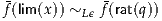 |
by the third constructor of ~.
This completes the (Rc, ~)-recursion, and hence the construction of . The desired equality (rat(q)) ≡ f(q) is exactly the first computation rule for (Rc, ~)-recursion, and the additional condition (11.3.13) says exactly that is Lipschitz with constant L. __
At this point we have gone about as far as we can without a better characterization of ~. We have specified, in the constructors of ~, the conditions under which we want Cauchy reals of the two different forms to be ϵ-close. However, how do we know that in the resulting inductive-inductive type family, these are the only witnesses to this fact? We have seen that inductive type families (such as identity types, see §5.8) and higher inductive types have a tendency to contain “more than was put into them”, so this is not an idle question.
In order to characterize ~ more precisely, we will define a family of relations ≈ϵ on Rc recursively, so that they will compute on constructors, and prove that this family is equivalent to ~ϵ.
Theorem 11.3.16. There is a family of mere relations ≈ : Rc →Rc →Q+ →Prop such that
Moreover, we have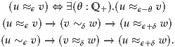 | (11.3.21) (11.3.22) (11.3.23) |
The additional conditions (11.3.21)–(11.3.23) turn out to be required in order to make the inductive definition go through. Condition (11.3.21) is called being rounded. Reading it from right to left gives monotonicity of ≈,
 |
while reading it left to right to openness of ≈,
 |
Conditions (11.3.22) and (11.3.23) are forms of the triangle inequality, which say that ≈ is a “module” over ~ on both sides.
Proof. We will define ≈ : Rc →Rc →Q+ →Prop by double (Rc, ~)-recursion.
First we will apply (Rc, ~)-recursion with codomain the subset of
Rc →Q+ →Prop consisting of those families of predicates which are
rounded and satisfy the one appropriate form of the triangle inequality.
Thinking of these predicates as half of a binary relation, we will write them as
(u, ϵ) (♢≈ϵu), with the symbol ♢ referring to the whole relation. Now we
can write A precisely as
(♢≈ϵu), with the symbol ♢ referring to the whole relation. Now we
can write A precisely as
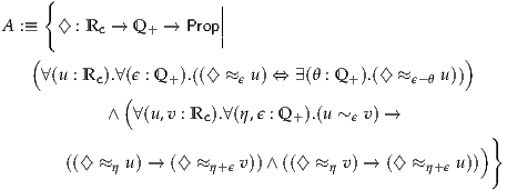 |
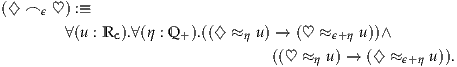
 |
to show ♢ = ♡ it suffices to show (♢≈ϵu) ⇔ (♡≈ϵu) for all u : Rc. But ♢≈ϵu implies ♢≈ϵ-θu for some θ, by roundedness, which together with ♢ ⌢ ϵ♡ implies ♡≈ϵu; and the converse is identical.
Now the first two data the recursion principle requires are the following.
 (xϵ ≈(–)–), with the property
that
(xϵ ≈(–)–), with the property
that
 | (11.3.24) |
we must give an element of A, which we write as (lim(x) ≈(–)–).
In both cases, we give the required definition by using a nested (Rc, ~)-recursion,
with codomain the subset of Q+ →Prop consisting of rounded families of
mere propositions. Thinking of these propositions as zero halves of a binary
relation, we will write them as ϵ (∙≈ϵ △), with the symbol △ referring to
the whole family. Now we can write the codomain of these inner recursions
precisely as
(∙≈ϵ △), with the symbol △ referring to
the whole family. Now we can write the codomain of these inner recursions
precisely as
 " class="math-display" >
Note that if such an inner recursion succeeds, it will yield a family of predicates ♢ : Rc →Q+ →Prop which are rounded (since their image in Q+ →Prop lies in C) and satisfy

Expanding out the definition of ⌣, this yields precisely the third condition for ♢ to belong to A; thus it is exactly what we need.
It is at this point that we can give the definitions (11.3.17)–(11.3.20), as the first two clauses of each of the two inner recursions, corresponding to rational points and limits. In each case, we must verify that the relation is rounded and hence lies in C. In the rational-rational case (11.3.17) this is clear, while in the other cases it follows from an inductive hypothesis. (In (11.3.18) the relevant inductive hypothesis is that (rat(q) ≈(–)yδ) : C, while in (11.3.19) and (11.3.20) it is that (xδ ≈(–)–) : A.)
The remaining data of the sub-recursions consist of showing that (11.3.17)–(11.3.20) satisfy the triangle inequality on the right with respect to the constructors of ~. There are eight cases — four in each sub-recursion — corresponding to the eight possible ways that u, v, and w in (11.3.22) can be chosen to be rational points or limits. First we consider the cases when u is rat(q).
 | (11.3.25) |
We assume also that ψ, δ (rat(q) ≈ψyδ) is a Cauchy approximation
with respect to ⌣, i.e.
(rat(q) ≈ψyδ) is a Cauchy approximation
with respect to ⌣, i.e.
 | (11.3.26) |
although we do not need this assumption in this case. Indeed, (11.3.25) with ψ :≡ ϕ yields immediately rat(q) ≈ϕ+ϵ-δyδ, and hence rat(q) ≈ϕ+ϵlim(y) by definition of ≈.
 | (11.3.27) (11.3.28) |
 | (11.3.29) (11.3.30) (11.3.31) |
Now we move on to the cases when u is lim(x), with x a Cauchy approximation. In this case, the ambient inductive hypothesis of the definition of (lim(x) ≈(–)–) : A is that we have (xδ ≈(–)–) : A, so that in addition to being rounded they satisfy the triangle inequality on the right.
This completes the two inner recursions, and thus the definitions of the families of relations (rat(q) ≈(–)–) and (lim(x) ≈(–)–). Since all are elements of A, they are rounded and satisfy the triangle inequality on the right with respect to ~. What remains is to verify the conditions relating to ⌢, which is to say that these relations satisfy the triangle inequality on the left with respect to the constructors of ~. The four cases correspond to the four choices of rational or limit points for u and v in (11.3.23), and since they are all mere propositions, we may apply Rc-induction and assume that w is also either rational or a limit. This yields another eight cases, whose proofs are essentially identical to those just given; so we will not subject the reader to them. __
We can now prove:
Proof. Since both are mere propositions, it suffices to prove bidirectional implication. For the left-to-right direction, we use ~-induction applied to C(u, v, ϵ) :≡ (u ≈ϵv). Thus, it suffices to consider the four constructors of ~. In each case, u and v are specialized to either rational points or limits, so that the definition of ≈ evaluates, and the inductive hypothesis always applies.
For the right-to-left direction, we use Rc-induction to assume that u and v are rational points or limits, allowing ≈ to evaluate. But now the definitions of ≈, and the inductive hypotheses, supply exactly the data required for the relevant constructors of ~. __
Stretching a point, one might call ≈ a fibration of “codes” for ~, with the two directions of the above proof being encode and decode respectively. By the definition of ≈, from Theorem 11.3.32 we get equivalences
| (rat(q) ~ϵ rat(r)) | = (-ϵ < q-r < ϵ) | ||
| (rat(q) ~ϵ lim(y)) | = ∃(δ : Q+).rat(q) ~ϵ-δ yδ | ||
| (lim(x) ~ϵ rat(r)) | = ∃(δ : Q+).xδ ~ϵ-δ rat(r) | ||
| (lim(x) ~ϵ lim(y)) | = ∃(δ, η : Q+).xδ ~ϵ-δ-η yη. |
With the triangle inequality in hand, we can show that “limits” of Cauchy approximations actually behave like limits.
Lemma 11.3.36. For any u : Rc, Cauchy approximation y, and ϵ, δ : Q+, if u ~ϵ yδ then u ~ϵ+δ lim(y).
Proof. We use Rc-induction on u. If u is rat(q), then this is exactly the second constructor of ~. Now suppose u is lim(x), and that each xη has the property that for any y, ϵ, δ, if xη ~ϵ yδ then xη ~ϵ+δ lim(y). In particular, taking y :≡ x and δ :≡ η in this assumption, we conclude that xη ~η+θ lim(x) for any η, θ : Q+.
Now let y, ϵ, δ be arbitrary and assume lim(x) ~ϵ yδ. By roundedness, there is a θ such that lim(x) ~ϵ-θ yδ. Then by the above observation, for any η we have xη ~η+θ/2 lim(x), and hence xη ~ϵ+η-θ/2 yδ by the triangle inequality. Hence, the fourth constructor of ~ yields lim(x) ~ϵ+2η+δ-θ/2 lim(y). Thus, if we choose η :≡ θ/4, the result follows. __
Proof. Take u :≡ yδ and ϵ :≡ η in the previous lemma. __
Remark 11.3.38. We might have expected to have yδ ~δ lim(y), but this fails in examples. For instance, consider x defined by xϵ :≡ ϵ. Its limit is clearly 0, but we do not have |ϵ- 0| < ϵ, only ≤.
As an application, Lemma 11.3.37 enables us to show that the extensions of Lipschitz functions from Lemma 11.3.15 are unique.
Lemma 11.3.39. Let f, g : Rc →Rc be continuous, in the sense that

and analogously for g. If f(rat(q)) = g(rat(q)) for all q : Q, then f = g.
Proof. We prove f(u) = g(u) for all u by Rc-induction. The rational case is just the hypothesis. Thus, suppose f(xδ) = g(xδ) for all δ. We will show that f(lim(x)) ~ϵ g(lim(x)) for all ϵ, so that the path constructor of Rc applies.
Since f and g are continuous, there exist θ, η such that for all v, we have
| (lim(x) ~θ v) | → (f(lim(x)) ~ϵ/2 f(v)) | ||
| (lim(x) ~η v) | → (g(lim(x)) ~ϵ/2 g(v)). |

and thus f(lim(x)) ~ϵ g(lim(x)) by the triangle inequality. __
We first define the additive structure (Rc, 0, +, -). Clearly, the additive unit element 0 is just rat(0), while the additive inverse - : Rc →Rc is obtained as the extension of the additive inverse - : Q →Q, using Lemma 11.3.15 with Lipschitz constant 1. We have to work a bit harder for addition.
Lemma 11.3.40. Suppose f : Q ×Q →Q satisfies, for all q, r, s : Q,
 |
Then there is a function : Rc ×Rc →Rc such that (rat(q), rat(r)) = f(q, r) for all q, r : Q. Furthermore, for all u, v, w : Rc and q : Q+,
 |
Proof. We use (Rc, ~)-recursion to construct the curried form of as a map Rc → A where A is the space of non-expanding real-valued functions:
 |
We shall also need a suitable ⌢ ϵ on A, which we define as
 |
Clearly, if ∀(ϵ : Q+).h ⌢ ϵk then h(u) = k(u) for all u : Rc, so ⌢ is separated.
For the base case we define (rat(q)) : A, where q : Q, as the extension of the Lipschitz map λr.f(q, r) from Q →Q to Rc →Rc, as constructed in Lemma 11.3.15 with Lipschitz constant 1. Next, for a Cauchy approximation x, we define (lim(x)) : Rc →Rc as
 |
For this to be a valid definition, λϵ.(xϵ)(v) should be a Cauchy approximation, so consider any δ, ϵ : Q. Then by assumption (xδ) ⌢ δ+ϵ(xϵ), hence (xδ)(v) ~δ+ϵ (xϵ)(v). Furthermore, (lim(x)) is non-expanding because (xϵ) is such by induction hypothesis. Indeed, if u ~ϵ v then, for all ϵ : Q,
 |
therefore (lim(x))(u) ~ϵ (lim(x))(v) by the fourth constructor of ~.
We still have to check four more conditions, let us illustrate just one. Suppose ϵ : Q+ and for some δ : Q+ we have rat(q) ~ϵ-δ yδ and (rat(q)) ⌢ ϵ-δ(yδ). To show (rat(q)) ⌢ ϵ(lim(y)), consider any v : Rc and observe that
 |
Therefore, by the second constructor of ~, we have
 |
as required. __
We may apply Lemma 11.3.40 to any bivariate rational function which is non-expanding separately in each variable. Addition is such a function, therefore we get + : Rc ×Rc →Rc. Furthermore, the extension is unique as long as we require it to be non-expanding in each variable, and just as in the univariate case, identities on rationals extend to identities on reals. Since composition of non-expanding maps is again non-expanding, we may conclude that addition satisfies the usual properties, such as commutativity and associativity. Therefore, (Rc, 0, +, -) is a commutative group.
We may also apply Lemma 11.3.40 to the functions min : Q ×Q →Q and max : Q ×Q →Q, which turns Rc into a lattice. The partial order ≤ on Rc is defined in terms of max as
 |
The relation ≤ is a partial order because it is such on Q, and the axioms of a partial order are expressible as equations in terms of min and max, so they transfer to Rc.
Another function which extends to Rc by the same method is the absolute value |–|. Again, it has the expected properties because they transfer from Q to Rc.
From ≤ we get the strict order < by
 |
That is, u < v holds when there merely exists a pair of rational numbers q < r such that x ≤rat(q) and rat(r) ≤ v. It is not hard to check that < is irreflexive and transitive, and has other properties that are expected for an ordered field. The archimedean principle follows directly from the definition of <.
Theorem 11.3.41 (Archimedean principle for Rc). For every u, v : Rc such that u < vthere merely exists q : Q such that u < q < v.
Proof. From u < v we merely get r, s : Q such that u ≤ r < s ≤ v, and we may take q :≡ (r + s)/2. __
We now have enough structure on Rc to express u ~ϵ v with standard concepts.
Lemma 11.3.42. If q : Q and u : Rc satisfy u ≤rat(q), then for any v : Rc and ϵ : Q+, if u ~ϵ vthen v ≤rat(q + ϵ).
Proof. Note that the function max(rat(q), –) : Rc →Rc is Lipschitz with constant 1. First consider the case when u = rat(r) is rational. For this we use induction on v. If v is rational, then the statement is obvious. If v is lim(y), we assume inductively that for any ϵ, δ, if rat(r) ~ϵ yδ then yδ ≤rat(q + ϵ), i.e. max(rat(q + ϵ), yδ) = rat(q + ϵ).
Now assuming ϵ and rat(r) ~ϵ lim(y), we have θ such that rat(r) ~ϵ-θ lim(y), hence rat(r) ~ϵ yδ whenever δ < θ. Thus, the inductive hypothesis gives max(rat(q + ϵ), yδ) = rat(q + ϵ) for such δ. But by definition,

Since the limit of an eventually constant Cauchy approximation is that constant, we have

hence lim(y) ≤rat(q + ϵ).
Now consider a general u : Rc. Since u ≤ rat(q) means max(rat(q), u) = rat(q), the assumption u ~ϵ v and the Lipschitz property of max(rat(q), -) imply max(rat(q), v) ~ϵ rat(q). Thus, since rat(q) ≤ rat(q), the first case implies max(rat(q), v) ≤ rat(q + ϵ), and hence v ≤rat(q + ϵ) by transitivity of ≤. __
Proof. By definition, u < rat(q) means there is r : Q with r < q and u ≤ rat(r). Then by Lemma 11.3.42, for any ϵ, if u ~ϵ v then v ≤rat(r + ϵ). Conclusion (i) follows immediately since r + ϵ < q + ϵ, while for (ii) we can take any ϵ < q-r. __
We are now able to show that the auxiliary relation ~ is what we think it is.
Proof. The Lipschitz properties of subtraction and absolute value imply that if u ~ϵ v, then |u-v| ~ϵ |u-u| = 0. Thus, for the left-to-right direction, it will suffice to show that if u ~ϵ 0, then |u| < rat(ϵ). We proceed by Rc-induction on u.
If u is rational, the statement follows immediately since absolute value and order extend the standard ones on Q+. If u is lim(x), then by roundedness we have θ : Q+ with lim(x) ~ϵ-θ 0. By the triangle inequality, therefore, we have xθ/3 ~ϵ-2θ/3 0, so the inductive hypothesis yields |xθ/3| < rat(ϵ- 2θ/3). But xθ/3 ~2θ/3 lim(x), hence |xθ/3| ~2θ/3 |lim(x)| by the Lipschitz property, so Lemma 11.3.43(i) implies |lim(x)| < rat(ϵ).
In the other direction, we use Rc-induction on u and v. If both are rational, this is the first constructor of ~.
If u is rat(q) and v is lim(y), we assume inductively that for any ϵ, δ, if |rat(q) - yδ| < rat(ϵ) then rat(q) ~ϵ yδ. Fix an ϵ such that |rat(q) -lim(y)| < rat(ϵ). Since Q is order-dense in Rc, there exists θ < ϵ with |rat(q) -lim(y)| < rat(θ). Now for any δ, η we have lim(y) ~2δ yδ, hence by the Lipschitz property

Thus, by Lemma 11.3.43(i), we have |rat(q) -yδ| < rat(θ + 2δ). So by the inductive hypothesis, rat(q) ~θ+2δ yδ, and thus rat(q) ~θ+4δ lim(y) by the triangle inequality. Thus, it suffices to choose δ :≡ (ϵ-θ)/4.
The remaining two cases are entirely analogous. __
Next, we would like to equip Rc with multiplicative
structure. For each q : Q the map r q⋅r is Lipschitz with
constant1
|q| + 1, and so we can extend it to multiplication by q on the real numbers.
Therefore Rc is a vector space over Q. In general, we can define multiplication
of real numbers as
q⋅r is Lipschitz with
constant1
|q| + 1, and so we can extend it to multiplication by q on the real numbers.
Therefore Rc is a vector space over Q. In general, we can define multiplication
of real numbers as
 | (11.3.45) |
so we just need squaring u u2 as a map Rc →Rc. Squaring is not a
Lipschitz map, but it is Lipschitz on every bounded domain, which
allows us to patch it together. Define the open and closed intervals
u2 as a map Rc →Rc. Squaring is not a
Lipschitz map, but it is Lipschitz on every bounded domain, which
allows us to patch it together. Define the open and closed intervals
![[u,v] :≡ {x : Rc|u ≤ x ≤ v} and (u,v) :≡ {x : Rc |u < x < v}.](hott-html4205x.png) |
Although technically an element of [u, v] or (u, v) is a Cauchy real number together with a proof, since the latter inhabits a mere proposition it is uninteresting. Thus, as is common with subset types, we generally write simply x : [u, v] whenever x : Rc is such that u ≤ x ≤ v, and similarly.
Theorem 11.3.46. There exists a unique function (–)2 : Rc →Rc which extends
squaring q q2 of rational numbers and satisfies
![2 2
∀(n : N).∀(u,v : [-n ,n]).|u - v | ≤ 2 ⋅n⋅|u- v|.](hott-html4207x.png) |
Proof. We first observe that for every u : Rc there merely exists n : N such that -n ≤ u ≤ n, see Exercise 11.7, so the map
![( )
e : ∑ [-n,n] → Rc defin ed by e(n,x) :≡ x
n:N](hott-html4210x.png) |
is surjective. Next, for each n : N, the squaring map
 |
is Lipschitz with constant 2n, so we can use Lemma 11.3.15 to extend it to a map n : [-n, n] →Rc with Lipschitz constant 2n, see Exercise 11.8 for details. The maps n are compatible: if m < n for some m, n : N then sn restricted to [-m, m] must agree with sm because both are Lipschitz, and therefore continuous in the sense of Lemma 11.3.39. Therefore, by Theorem 10.1.5 the map
![( )
∑ [-n,n] → Rc, givenby (n,x) ↦→ sn(x)
n:N](hott-html4214x.png) |
factors uniquely through Rc to give us the desired function. __
At this point we have the ring structure of the reals and the archimedean order. To establish Rc as an archimedean ordered field, we still need inverses.
Proof. First, suppose u : Rc has an inverse v : Rc By the archimedean principle there is q : Q such that |v| < q. Then 1 = |uv| < |u|⋅v < |u|⋅q and hence |u| > 1/q, which is to say that u # 0.
For the converse we construct the inverse map
 |
by patching together functions, similarly to the construction of squaring in Theorem 11.3.46. We only outline the main steps. For every q : Q let
![[q,∞) :≡ {u : Rc|q ≤ u} and (- ∞ ,q] :≡ {u : Rc|u ≤ -q}.](hott-html4218x.png) |
Then, as q ranges over Q+, the types (-∞, q] and [q, ∞) jointly cover
 u # 0}. On each such [q, ∞) and (-∞, q] the inverse function is
obtained by an application of Lemma 11.3.15 with Lipschitz constant 1/q2.
Finally, Theorem 10.1.5 guarantees that the inverse function factors uniquely
through
u # 0}. On each such [q, ∞) and (-∞, q] the inverse function is
obtained by an application of Lemma 11.3.15 with Lipschitz constant 1/q2.
Finally, Theorem 10.1.5 guarantees that the inverse function factors uniquely
through  u # 0}. __
We summarize the algebraic structure of Rc with a theorem.
We constructed Rc by closing Q under limits of Cauchy approximations, so it better be the case that Rc is Cauchy complete. Thanks to Theorem 11.3.44 there is no difference between a Cauchy approximation x : Q+ →Rc as defined in the construction of Rc, and a Cauchy approximation in the sense of Definition 11.2.10 (adapted to Rc).
Thus, given a Cauchy approximation x : Q+ →Rc it is quite natural to expect that lim(x) is its limit, where the notion of limit is defined as in Definition 11.2.10. But this is so by Theorem 11.3.44 and Lemma 11.3.37. We have proved:
An archimedean ordered field in which every Cauchy approximation has a limit is called Cauchy complete. The Cauchy reals are the least such field.
Proof. Suppose F is a Cauchy complete archimedean ordered field. Because limits are unique, there is an operator lim which takes Cauchy approximations in F to their limits. We define the embedding e : Rc → F by (Rc, ~)-recursion as
 |
A suitable ⌢ on F is
 |
This is a separated relation because F is archimedean. The rest of the clauses for (Rc, ~)-recursion are easily checked. One would also have to check that e is an embedding of ordered fields which fixes the rationals. __
Let us also say something about the relationship between the Cauchy and Dedekind reals. By Theorem 11.3.48, Rc is an archimedean ordered field. It is also admissible for Ω, as can be easily checked. (In case Ω is the initial σ-frame it takes a simple induction, while in other cases it is immediate.) Therefore, by Theorem 11.2.14 there is an embedding of ordered fields
 |
which fixes the rational numbers. (We could also obtain this from Theorems 11.2.12 and 11.3.50.) In general we do not expect Rc and Rd to coincide without further assumptions.
Lemma 11.4.1. If for every x : Rd there merely exists
 | (11.4.2) |
then the Cauchy and Dedekind reals coincide.
Proof. Note that the type in (11.4.2) is an untruncated variant of (11.2.3), which states that < is a weak linear order. We already know that Rc embeds into Rd, so it suffices to show that every Dedekind real merely is the limit of a Cauchy sequence of rational numbers.
Consider any x : Rd. By assumption there merely exists c as in the
statement of the lemma, and by inhabitation of cuts there merely exist a, b : Q
such that a < x < b. We construct a sequence f : N → q < r}
by recursion:
q < r}
by recursion:
Let us write (qn, rn) for the n-th term of the sequence f. Then it is easy to see that qn < x < rn and |qn-rn|≤ (2/3)n⋅|q0 -r0| for all n : N. Therefore q0, q1, … and r0, r1, … are both Cauchy sequences converging to the Dedekind cut x. We have shown that for every x : Rd there merely exists a Cauchy sequence converging to x. __
The lemma implies that either countable choice or excluded middle suffice for coincidence of Rc and Rd.
Proof. If excluded middle holds then (x < y) → (x < z)+(z < y) can be proved: either x < z or ¬(x < z). In the former case we are done, while in the latter we get z < y because z ≤ x < y. Therefore, we get (11.4.2) so that we can apply Lemma 11.4.1.
Suppose countable choice holds. The set S =  q < r} is
equivalent to N, so we may apply countable choice to the statement that x is
located,
q < r} is
equivalent to N, so we may apply countable choice to the statement that x is
located,
 |
Note that (q < x) ∨ (x < r) is expressible as an existential statement ∃(b : 2).(b = 02 → q < x) ∧ (b = 12 → x < r). The (curried form) of the choice function is then precisely (11.4.2) so that Lemma 11.4.1 is applicable again. __
We already pointed out that our constructions of reals are entirely compatible with classical logic. Thus, by assuming the law of excluded middle (3.4.1) and the axiom of choice (3.8.1) we could develop classical analysis, which would essentially amount to copying any standard book on analysis.
Nevertheless, anyone interested in computation, for example a numerical analyst, ought to be curious about developing analysis in a computationally meaningful setting. That analysis in a constructive setting is even possible was demonstrated by [Bis67]. As a sample of the differences and similarities between classical and constructive analysis we shall briefly discuss just one topic—compactness of the closed interval [0, 1] and a couple of theorems surrounding the concept.
Compactness is no exception to the common phenomenon in constructive mathematics that classically equivalent notions bifurcate. The three most frequently used notions of compactness are:
These are all equivalent in classical mathematics. Let us see how they fare in homotopy type theory. We can use either the Dedekind or the Cauchy reals, so we shall denote the reals just as R. We first recall several basic definitions.
Definition 11.5.1. A metric space (M, d) is a set M with a map d : M×M →R satisfying, for all x, y, z : M,
| d(x, y) | ≥ 0, | d(x, y) | = d(y, x), | ||||
| d(x, y) | = 0 ⇔ x = y, | d(x, z) | ≤ d(x, y) + d(y, z). |
Definition 11.5.2. A Cauchy approximation in M is a sequence x : Q+ → M satisfying
 |
The limit of a Cauchy approximation x : Q+ → M is a point ℓ : M satisfying
 |
A complete metric space is one in which every Cauchy approximation has a limit.
Definition 11.5.3. For a positive rational ϵ, an ϵ-net in a metric space (M, d) is an element of
 |
In words, this is a finite sequence of points x1, …, xn such that every point in M merely is within ϵ of some xk.
A metric space (M, d) is totally bounded when it has ϵ-nets of all sizes:
 |
Remark 11.5.4. In the definition of total boundedness we used sloppy notation ∑(n:N) ∑(x1,...,xn:M) . Formally, we should have written ∑ (x:List(M)) instead, where List(M) is the inductive type of finite lists from §5.1. However, that would make the rest of the statement a bit more cumbersome to express.
Note that in the definition of total boundedness we require pure existence of an ϵ-net, not mere existence. This way we obtain a function which assigns to each ϵ : Q+ a specific ϵ-net. Such a function might be called a “modulus of total boundedness”. In general, when porting classical metric notions to homotopy type theory, we should use propositional truncation sparingly, typically so that we avoid asking for a non-constant map from R to Q or N. For instance, here is the “correct” definition of uniform continuity.
Definition 11.5.5. A map f : M →R on a metric space is uniformly continuous when
 |
In particular, a uniformly continuous map has a modulus of uniform continuity, which is a function that assigns to each ϵ a corresponding δ.
Let us show that [0, 1] is compact in the first sense.
Proof. Given ϵ : Q+, there is n : N such that 2/k < ϵ, so we may take the ϵ-net xi = i/k for i = 0, …, k- 1. This is an ϵ-net because, for every y : [0, 1] there merely exists i such that 0 ≤ i < k and (i- 1)/k < y < (i + 1)/k, and so |y-xi| < 2/k < ϵ.
For completeness of [0, 1], consider a Cauchy approximation x : Q+ → [0, 1] and let ℓ be its limit in R. Since max and min are Lipschitz maps, the retraction r : R → [0, 1] defined by r(x) :≡ max(0, min(1, x)) commutes with limits of Cauchy approximations, therefore
 |
which means that 0 ≤ ℓ ≤ 1, as required. __
We thus have at least one good notion of compactness in homotopy type theory. Unfortunately, it is limited to metric spaces because total boundedness is a metric notion. We shall consider the other two notions shortly, but first we prove that a uniformly continuous map on a totally bounded space has a supremum, i.e. an upper bound which is less than or equal to all other upper bounds.
Theorem 11.5.7. A uniformly continuous map f : M → R on a totally bounded metric space (M, d) has a supremum m : R. For every ϵ : Q+ there exists u : M such that |m-f(u)| < ϵ.
Proof. Let h : Q+ →Q+ be the modulus of uniform continuity of f. We define an approximation x : Q+ →R as follows: for any ϵ : Q total boundedness of M gives a h(ϵ)-net y0, …, yn. Define
 |
We claim that x is a Cauchy approximation. Consider any ϵ, η : Q, so that
 |
for some h(ϵ)-net y0, …, yn and h(η)-net z0, …, zm. Every zi is merely h(ϵ)-close to some yj, therefore |f(zi) -f(yj)| < ϵ, from which we may conclude that
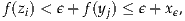 |
therefore xη < ϵ + xϵ. Symmetrically we obtain xη < η + xη, therefore |xη -xϵ| < η + ϵ.
We claim that m :≡ lim x is the supremum of f. To prove that f(x) ≤ m for all x : M it suffices to show ¬(m < f(x)). So suppose to the contrary that m < f(x). There is ϵ : Q+ such that m + ϵ < f(x). But now merely for some yi participating in the definition of xϵ we get |f(x) -f(yi) < ϵ, therefore m < f(x) -ϵ < f(yi) ≤ m, a contradiction.
We finish the proof by showing that m satisfies the second part of the theorem, because it is then automatically a least upper bound. Given any ϵ : Q+, on one hand |m-f(xϵ/2)| < 3ϵ/4, and on the other |f(xϵ/2) -f(yi)| < ϵ/4 merely for some yi participating in the definition of xϵ/2, therefore by taking u :≡ yi we obtain |m-f(u)| < ϵ by triangle inequality. __
Now, if in Theorem 11.5.7 we also knew that M were complete, we could hope to weaken the assumption of uniform continuity to continuity, and strengthen the conclusion to existence of a point at which the supremum is attained. The usual proofs of these improvements rely on the facts that in a complete totally bounded space
The first statement follows easily from Heine-Borel compactness, and the second is just Bolzano–Weierstraß compactness. Unfortunately, these are both somewhat problematic. Let us first show that Bolzano–Weierstraß compactness implies an instance of excluded middle known as the limited principle of omniscience: for every α : N →2,
 | (11.5.8) |
Computationally speaking, we would not expect this principle to hold, because it asks us to decide whether infinitely many values of a function are 02.
Theorem 11.5.9. Bolzano–Weierstraß compactness of [0, 1] implies the limited principle of omniscience.
Proof. Given any α : N →2, define the sequence x : N → [0, 1] by
 |
If the Bolzano–Weierstraß property holds, there exists a strictly increasing f : N →N such that x∘f is a Cauchy sequence. For a sufficiently large n : N the n-th term xf(n) is within 1/6 of its limit. Either xf(n) < 2/3 or xf(n) > 1/3. If xf(n) < 2/3 then xn converges to 0 and so ∏(n:N) α(n) = 02. If xf(n) > 1/3 then xf(n) = 1, therefore ∑(n:N) α(n) = 12. __
While we might not mourn Bolzano–Weierstraß compactness too much, it seems harder to live without Heine–Borel compactness, as attested by the fact that both classical mathematics and Brouwer’s Intuitionism accepted it. As we do not want to wade too deeply into general topology, we shall work with basic open sets. In the case of R these are the open intervals with rational endpoints. A family of such intervals, indexed by a type I, would be a map
 |
with the idea that a pair of rationals (q, r) with q < r determines the type
 q < x < r}. It is slightly more convenient to allow degenerate intervals
as well, so we take a family of basic intervals to be a map
q < x < r}. It is slightly more convenient to allow degenerate intervals
as well, so we take a family of basic intervals to be a map
 |
To be quite precise, a family is a dependent pair (I,  ), not just . A finite
family of basic intervals is one indexed by
), not just . A finite
family of basic intervals is one indexed by  m < n} for some n : N.
We usually present it by a finite list [(q0, r0), …, (qn-1, rn-1)]. Finally, a finite
subfamily of (I, ) is given by a list of indices [i1, …, in] which then determine
the finite family [(i1), …, (in)].
m < n} for some n : N.
We usually present it by a finite list [(q0, r0), …, (qn-1, rn-1)]. Finally, a finite
subfamily of (I, ) is given by a list of indices [i1, …, in] which then determine
the finite family [(i1), …, (in)].
As long as we are aware of the distinction between a pair (q, r) and the
corresponding interval  q < x < r}, we may safely use the same
notation (q, r) for both. Intersections and inclusions of intervals are
expressible in terms of their endpoints:
q < x < r}, we may safely use the same
notation (q, r) for both. Intersections and inclusions of intervals are
expressible in terms of their endpoints:
| (q, r) ∩ (s, t) | :≡ (max(q, s), min(r, t)), | ||
| (q, r) ⊆ (s, t) | :≡ (q < r ⇒ s ≤ q < r ≤ t). |
![∀(x : [a,b]).∃(i : I).qi < x < ri.](hott-html4278x.png) | (11.5.10) |
The Heine-Borel compactness for [0, 1] states that every covering family of [0, 1] merely has a finite subfamily which still covers [0, 1].
Proof. Assume for the purpose of reaching a contradiction that a family (I, λi.(ai, bi)) covers [0, 1] but no finite subfamily does. We construct a sequence of closed intervals [qn, rn] which are nested, their sizes shrink to 0, and none of them is covered by a finite subfamily of (I, λi.(ai, bi)).
We set [q0, r0] :≡ [0, 1]. Assuming [qn, rn] has been constructed, let s :≡ (2qn + rn)/3 and t :≡ (qn + 2rn)/3. Both [qn, t] and [s, rn] are covered by (I, λi.(ai, bi)), but they cannot both have a finite subcover, or else so would [qn, rn]. Either [qn, t] has a finite subcover or it does not. If it does we set [qn+1, rn+1] :≡ [s, rn], otherwise we set [qn+1, rn+1] :≡ [qn, t].
The sequences q0, q1, … and r0, r1, … are both Cauchy and they converge to a point x : [0, 1] which is contained in every [qn, rn]. There merely exists i : I such that ai < x < bi. Because the sizes of the intervals [qn, rn] shrink to zero, there is n : N such that ai < qn ≤ x ≤ rn < bi, but this means that [qn, rn] is covered by a single interval (ai, bi), while at the same time it has no finite subcover. A contradiction. __
Without excluded middle, or a pinch of Brouwerian Intuitionism, we seem to be stuck. Nevertheless, Heine-Borel compactness of [0, 1] can be recovered in a constructive setting, in a fashion that is still compatible with classical mathematics! For this to be done, we need to revisit the notion of cover. The trouble with (11.5.10) is that the truncated existential allows a space to be covered in any haphazard way, and so computationally speaking, we stand no chance of merely extracting a finite subcover. By removing the truncation we get
![∏ ∑ qi < x < ri,
(x:[0,1])(i:I)](hott-html4281x.png) | (11.5.12) |
which might help, were it not too demanding of covers. With this definition we could not even show that (0, 3) and (2, 5) cover [1, 4] because that would amount to exhibiting a non-constant map [1, 4] →2, see Exercise 11.6. Here we can take a lesson from “pointfree topology” (i.e. locale theory): the notion of cover ought to be expressed in terms of open sets, without reference to points. Such a “holistic” view of space will then allow us to analyze the notion of cover, and we shall be able to recover Heine-Borel compactness. Locale theory uses power sets, which we could obtain by assuming propositional resizing; but instead we can steal ideas from the predicative cousin of locale theory, which is called “formal topology”.
Suppose that we have a family (I, ) and an interval (a, b). How might we
express the fact that (a, b) is covered by the family, without referring to
points? Here is one: if (a, b) equals some (i) then it is covered by the family.
And another one: if (a, b) is covered by some other family (J,  ), and in turn
each (j) is covered by (I, ), then (a, b) is covered (I, ). Notice that we are
listing rules which can be used to deduce that (I, ) covers (a, b). We
should find sufficiently good rules and turn them into an inductive
definition.
), and in turn
each (j) is covered by (I, ), then (a, b) is covered (I, ). Notice that we are
listing rules which can be used to deduce that (I, ) covers (a, b). We
should find sufficiently good rules and turn them into an inductive
definition.
Definition 11.5.13. The inductive cover ⊲is a mere relation
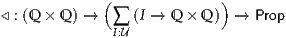 |
defined inductively by the following rules, where q, r, s, t are rational numbers
and (I, ), (J, ) are families of basic intervals:
(i) ⊲ (I, ) for all i : I,
) and ∀(j : J).(j) ⊲ (I, ) then (q, r) ⊲
(I, ),
) then (q, r) ⊲ (I, ),
) then (q, r)∩(s, t)⊲(I, λi.((i)∩(s, t))).
 q < s < t < r}, λu.u).
The definition should be read as a higher-inductive type in which the listed rules are point constructors, and the type is (-1)-truncated. The first four clauses are of a general nature and should be intuitively clear. The last two clauses are specific to the real line: one says that an interval may be covered by two intervals if they overlap, while the other one says that an interval may be covered from within. Incidentally, if r ≤ q then (q, r) is covered by the empty family by the last clause.
Inductive covers enjoy the Heine-Borel property, the proof of which requires a lemma.
Lemma 11.5.14. Suppose q < s < t < r and (q, r) ⊲ (I, ). Then there
merely exists a finite subfamily of (I, ) which inductively covers (s, t).
Proof. We prove the statement by induction on (q, r) ⊲ (I, ). There are six
cases:
(i) then by monotonicity (s, t) is covered
by the finite subfamily [(i)].
) and ∀(j : J).(j) ⊲ (I, ). By
the inductive hypothesis there merely exists [(j1), …, (jn)] which
covers (s, t). Again by the inductive hypothesis, each of (jk) is
covered by a finite subfamily of (I, ), and we can collect these
into a finite subfamily which covers (s, t).
) then we may
apply the inductive hypothesis to (u, v) ⊲ (I, ) because u < s <
t < v.
) and (q, r) = (q′, r′) ∩ (a, b).
Because q′ < s < t < r′, by the inductive hypothesis there
is a finite subcover [(i1), …, (in)] of (s, t). We also know that
a < s < t < b, therefore (s, t) = (s, t) ∩ (a, b) is covered
by [(i1) ∩ (a, b), …, (in) ∩ (a, b)], which is a finite subfamily of
(I, λi.((i) ∩ (a, b))).
 q < u < v < r}, λz.z) by reflexivity.
__
q < u < v < r}, λz.z) by reflexivity.
__ Say that (I, ) inductively covers [a, b] when there merely exists ϵ : Q+
such that (a-ϵ, b + ϵ) ⊲ (I, ).
Proof. Suppose [a, b] is inductively covered by (I, ), so there merely is
ϵ : Q+ such that (a-ϵ, b + ϵ) ⊲ (I, ). By Lemma 11.5.14 there is a finite
subcover of (a-ϵ/2, b + ϵ/2), which is therefore a finite subcover of
[a, b]. __
Experience from formal topology shows that the rules for inductive covers are sufficient for a constructive development of pointfree topology. But we can also provide our own evidence that they are a reasonable notion.
Proof.
), where we write
(qi, ri) :≡(i), an interval (a, b) inductively covered by (I, ), and
x such that a < x < b. We prove by induction on (a, b) ⊲ (I, )
that there merely exists i : I such that qi < x < ri. Most cases are
pretty obvious, so we show just two. If (a, b) ⊲ (I, ) by reflexivity,
then there merely is some i : I such that (a, b) = (qi, ri) and so
qi < x < ri. If (a, b) ⊲ (I, ) by transitivity via (J, λj.(sj, tj)) then by
the inductive hypothesis there merely is j : J such that sj < x < tj,
and then since (sj, tj) ⊲ (I, ) again by the inductive hypothesis
there merely exists i : I such that qi < x < ri. Other cases are just
as exciting.
 |
The intervals (c0, c2), (c1, c3), …, (ck-2, ck) inductively cover (c, d) by repeated use of transitivity and Item (v) in Definition 11.5.13. Because their widths are below ϵ each of them is contained in some (qi, ri), and we may use transitivity and monotonicity to conclude that (I, λi.(qi, ri)) inductively cover (c, d). __
The upshot of the previous theorem is that, as far as classical mathematics is concerned, there is no difference between a pointwise and an inductive cover. In particular, since it is consistent to assume excluded middle in homotopy type theory, we cannot exhibit an inductive cover which fails to be a pointwise cover. Or to put it in a different way, the difference between pointwise and inductive covers is not what they cover but in the proofs that they cover.
We could write another book by going on like this, but let us stop here and hope that we have provided ample justification for the claim that analysis can be developed in homotopy type theory. The curious reader should consult Exercise 11.13 for constructive versions of the mean value theorem.
In this section we consider another example of a higher inductive-inductive
type, which draws together many of our threads: Conway’s field No of surreal
numbers [Con76]. The surreal numbers are the natural common generalization
of the (Dedekind) real numbers (§11.2) and the ordinal numbers (§10.3).
Conway, working in classical mathematics with excluded middle and Choice,
defines a surreal number to be a pair of sets of surreal numbers, written
{L R}, such that every element of L is strictly less than every element of R.
This obviously looks like an inductive definition, but there are three issues
with regarding it as such.
R}, such that every element of L is strictly less than every element of R.
This obviously looks like an inductive definition, but there are three issues
with regarding it as such.
Firstly, the definition requires the relation of (strict) inequality between surreals, so that relation must be defined simultaneously with the type No of surreals. (Conway avoids this issue by first defining games, which are like surreals but omit the compatibility condition on L and R.) As with the relation ~ for the Cauchy reals, this simultaneous definition could a priori be either inductive-inductive or inductive-recursive. We will choose to make it inductive-inductive, for the same reasons we made that choice for ~.
Moreover, we will define strict inequality < and non-strict inequality ≤ for surreals separately (and mutually inductively). Conway defines < in terms of ≤, in a way which is sensible classically but not constructively. Furthermore, a negative definition of < would make it unacceptable as a hypothesis of the constructor of a higher inductive type (see §5.6).
Secondly, Conway says that L and R in {L R} should be “sets of surreal
numbers”, but the naive meaning of this as a predicate No →Prop is not
positive, hence cannot be used as input to an inductive constructor. However,
this would not be a good type-theoretic translation of what Conway means
anyway, because in set theory the surreal numbers form a proper class,
whereas the sets L and R are true (small) sets, not arbitrary subclasses of No.
In type theory, this means that No will be defined relative to a universe , but
will itself belong to the next higher universe ′, like the sets Ord and
Card of ordinals and cardinals, the cumulative hierarchy V , or even
the Dedekind reals in the absence of propositional resizing. We will
then require the “sets” L and R of surreals to be -small, and so it
is natural to represent them by families of surreals indexed by some
-small type. (This is all exactly the same as what we did with the
cumulative hierarchy in §10.5.) That is, the constructor of surreals will have
type
R} should be “sets of surreal
numbers”, but the naive meaning of this as a predicate No →Prop is not
positive, hence cannot be used as input to an inductive constructor. However,
this would not be a good type-theoretic translation of what Conway means
anyway, because in set theory the surreal numbers form a proper class,
whereas the sets L and R are true (small) sets, not arbitrary subclasses of No.
In type theory, this means that No will be defined relative to a universe , but
will itself belong to the next higher universe ′, like the sets Ord and
Card of ordinals and cardinals, the cumulative hierarchy V , or even
the Dedekind reals in the absence of propositional resizing. We will
then require the “sets” L and R of surreals to be -small, and so it
is natural to represent them by families of surreals indexed by some
-small type. (This is all exactly the same as what we did with the
cumulative hierarchy in §10.5.) That is, the constructor of surreals will have
type

which is indeed strictly positive.
Finally, after giving the mutual definitions of No and its ordering, Conway
declares two surreal numbers x and y to be equal if x ≤ y and y ≤ x. This is
naturally read as passing to a quotient of the set of “pre-surreals” by an
equivalence relation. However, in the absence of the axiom of choice, such a
quotient presents the same problem as the quotient in the usual construction
of Cauchy reals: it will no longer be the case that a pair of families of surreals
yield a new surreal {L R}, since we cannot necessarily “lift” L and R to
families of pre-surreals. Of course, we can solve this problem in the same
way we did for Cauchy reals, by using a higher inductive-inductive
definition.
R}, since we cannot necessarily “lift” L and R to
families of pre-surreals. Of course, we can solve this problem in the same
way we did for Cauchy reals, by using a higher inductive-inductive
definition.
Definition 11.6.1. The type No of surreal numbers, along with the
relations < : No →No → and ≤ : No →No →, are defined higher
inductive-inductively as follows. The type No has the following constructors.
 , : and functions → No and → No, whose
values we write as xL and xR for L : and R : respectively, if
∀(L : ).∀(R : ).xL < xR, then there is a surreal number x.
, : and functions → No and → No, whose
values we write as xL and xR for L : and R : respectively, if
∀(L : ).∀(R : ).xL < xR, then there is a surreal number x.
We will refer to the inputs of the first constructor as a cut. If x is the surreal
number constructed from a cut, then the notation xL will implicitly assume
L : , and similarly xR will assume R : . In this way we can usually avoid
naming the indexing types and , which is convenient when there are
many different cuts under discussion. Following Conway, we call xL a left
option of x and xR a right option.
The path constructor implies that different cuts can define the same surreal number. Thus, it does not make sense to speak of the left or right options of an arbitrary surreal number x, unless we also know that x is defined by a particular cut. Thus in what follows we will say, for instance, “given a cut defining a surreal number x” in contrast to “given a surreal number x”.
The relation ≤ has the following constructors.
And the relation < has the following constructors.
We compare this with Conway’s definitions:
 R}. All numbers are constructed in this way.
The inclusion of x ≥ y in the definition of x > y is unnecessary if all objects are
[surreal] numbers rather than “games”. Thus, Conway’s < is just the negation
of his ≥, so that his condition for {L R} to be a surreal is the same as ours.
Negating Conway’s ≤ and canceling double negations, we arrive at our
definition of <, and we can then reformulate his ≤ in terms of < without
negations.
R} to be a surreal is the same as ours.
Negating Conway’s ≤ and canceling double negations, we arrive at our
definition of <, and we can then reformulate his ≤ in terms of < without
negations.
We can immediately populate No with many surreal numbers. Like Conway, we write
for the surreal number defined by a cut where →No and →No are
families described by x, y, z, … and u, v, w, …. Of course, if or are 0, we
leave the corresponding part of the notation empty. There is an unfortunate
clash with the standard notation  P(x)} for subsets, but we will not use
the latter in this section.
P(x)} for subsets, but we will not use
the latter in this section.
| ιN(0) | :≡{ }, }, | ||
| ιN(succ(n)) | :≡{ιN(n) }. }. |
| ιZ(0) | :≡{ }, }, | ||||||
| ιZ(n + 1) | :≡{ιZ(n) } } | n ≥ 0, | |||||
| ιZ(n- 1) | :≡{ ιZ(n)} ιZ(n)} | n ≤ 0. |
| ιQD(a/20) | :≡ ιZ(a), | ||
| ιQD(a/2n) | :≡{a/2n - 1/2n a/2n + 1/2n}, for n > 0. a/2n + 1/2n}, for n > 0. |
| ιRd(x) | :≡{q ∈QD such that q < x q ∈QD such that x < q}. q ∈QD such that x < q}. |
 " class="math-display" >
 |
It will also follow from the simplicity theorem that ιOrd restricted to finite ordinals agrees with ιN.
| ω | :≡{0, 1, 2, 3, … } (also an ordinal) } (also an ordinal) | ||
| -ω | :≡{ …, -3, -2, -1, 0} …, -3, -2, -1, 0} | ||
| 1/ω | :≡{0 1, 1,  , ,  , ,  , …} , …} | ||
| ω- 1 | :≡{0, 1, 2, 3, … ω} ω} | ||
| ω/2 | :≡{0, 1, 2, 3, … …, ω- 2, ω- 1, ω}. …, ω- 2, ω- 1, ω}. |
In identifying surreal numbers presented by different cuts, the following simple observation is useful.
Theorem 11.6.2 (Conway’s simplicity theorem). Suppose x and zare surreal numbers defined by cuts, and that the following hold.
Then x = z.
Proof. Applying the path constructor of No, we must show x ≤ z and z ≤ x. The first entails showing xL < z for all L, which we assumed, and x < zR for all R. But by assumption, for any zR there is an xR′ with xR′ ≤ zR hence x < zR as desired. Thus x ≤ z; the proof of z ≤ x is symmetric. __
In order to say much more about surreal numbers, however, we need their induction principle. The mutual induction principle for (No, ≤, <) applies to three families of types:
| A | : No → | ||
| B | : ∏
(x,y:No) ∏
(a:A(x)) ∏
(b:A(y)) (x ≤ y) → | ||
| C | : ∏
(x,y:No) ∏
(a:A(x)) ∏
(b:A(y)) (x < y) →. |
there is a specified element fa : A(x). We call such data a dependent cut over the cut defining x.
Under these hypotheses we deduce a function f : ∏(x:No) A(x) such that
| f(x) | ≡ff[x] | (11.6.3) | |
| (x ≤ y) | ⇒(x, f(x)) ⊴ (y, f(y)) | ||
| (x < y) | ⇒(x, f(x)) ◃ (y, f(y)). |
 xR} may use the symbols f(xL) and f(xR) and the assumption that they
form a dependent cut.
xR} may use the symbols f(xL) and f(xR) and the assumption that they
form a dependent cut.
As with the Cauchy reals, we have special cases resulting from trivializing some of A, ⊴, and ◃. Taking ⊴ and ◃ to be constant at 1, we have No-induction, which for simplicity we state only for mere properties:
This should be compared with Conway’s remark:
In general when we wish to establish a proposition P(x) for all numbers x, we will prove it inductively by deducing P(x) from the truth of all the propositions P(xL) and P(xR). We regard the phrase “all numbers are constructed in this way” as justifying the legitimacy of this procedure.
With No-induction, we can prove
Proof. Note first that if x ≤ x, then whenever x occurs as a left option of some cut y, we have x < y by the first constructor of <, and similarly whenever x occurs as a right option of a cut y, we have y < x by the second constructor of <. In particular, (i)⇒(ii).
We prove (i) by No-induction on x. Thus, assume x is defined by a cut such that xL ≤ xL and xR ≤ xR for all L and R. But by our observation above, these assumptions imply xL < x and x < xR for all L and R, yielding x ≤ x by the constructor of ≤. __
Proof. The mere relation R(x, y) :≡ (x ≤ y) ∧ (y ≤ x) implies identity by the path constructor of No, and contains the diagonal by Theorem 11.6.4(i). Thus, Theorem 7.2.2 applies. __
By contrast, Conway’s Theorem 1 (transitivity of ≤) is somewhat harder to establish with our definition; see Corollary 11.6.17.
We will also need the joint recursion principle, (No, ≤, <)-recursion, which it is convenient to state as follows. Suppose A is a type equipped with relations ⊴ : A → A →Prop and ◃ : A → A →Prop. Then we can define f : No → A by doing the following.
The last three clauses can be more concisely described by saying we must prove that f (as defined in the first clause) takes ≤ to ⊴ and < to ◃. We will refer to these properties by saying that f preserves inequalities. Moreover, in proving that f preserves inequalities, we may assume the particular instance of ≤ or < to be obtained from one of its constructors, and we may also use inductive hypotheses that f preserves all inequalities appearing in the input to that constructor.
If we succeed at (i)–(v) above, then we obtain f : No → A, which computes on cuts as specified by (i), and which preserves all inequalities:
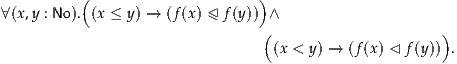
Example 11.6.6. Let us define the negation function No →No. We apply the joint recursion principle with A :≡No, with (x ⊴ y) :≡ (y ≤ x), and (x ◃ y) :≡ (y < x). Clearly this ⊴ is antisymmetric.
For the main clause in the definition, we assume x defined by a cut,
with -xL and -xR defined such that -xL ◃ -xR for all L and R. By
definition, this means -xR < -xL for all L and R, so we can define -x
by the cut {-xR -xL}. This notation, which follows Conway, refers
to the cut whose left options are indexed by the type indexing the
right options of x, and whose right options are indexed by the type
indexing the left options of x, with the corresponding families →No
and →No defined by composing those for x with negation.
-xL}. This notation, which follows Conway, refers
to the cut whose left options are indexed by the type indexing the
right options of x, and whose right options are indexed by the type
indexing the left options of x, with the corresponding families →No
and →No defined by composing those for x with negation.
We now have to verify that f preserves inequalities.
To do much more than this, however, we will need to characterize the relations ≤ and < more explicitly, as we did for the Cauchy reals in Theorem 11.3.32. Also as there, we will have to simultaneously prove a couple of essential properties of these relations, in order for the induction to go through.
Theorem 11.6.7. There are relations ≼ : No →No →Prop and ≺ : No →No →Prop such that if x and y are surreals defined by cuts, then
| (x ≼ y) | :≡ ∀(L).xL ≺ y ∀(L).xL ≺ y ∧ ∧ ∀(R).x ≺ yR ∀(R).x ≺ yR | ||
| (x ≺ y) | :≡ ∃(L).x ≼ yL ∃(L).x ≼ yL ∨ ∨ ∃(R).xR ≼ y ∃(R).xR ≼ y . . |
 | (11.6.8) |
and all the reasonable transitivity properties making ≺and ≼into a “bimodule” over ≤and <:
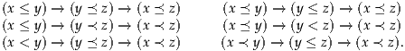 | (11.6.9) |
Proof. We define ≼ and ≺ by double (No, ≤, <)-induction on x, y. The first
induction is a simple recursion, whose codomain is the subset A of
(No →Prop) × (No →Prop) consisting of pairs of predicates of which one
implies the other and which satisfy “transitivity on the right”, i.e. (11.6.8) and
the right column of (11.6.9) with (x ≼ –) and (x ≺ –) replaced by the two
given predicates. As in the proof of Theorem 11.3.16, we regard these
predicates as half of binary relations, writing them as y (♢≼ y) and
y
(♢≼ y) and
y (♢≺ y), with ♢ denoting the pair of relations. We equip A with the
following two relations:
(♢≺ y), with ♢ denoting the pair of relations. We equip A with the
following two relations:
| (♢⊴♡) | :≡∀(y : No). (♡≼ y) → (♢≼ y) (♡≼ y) → (♢≼ y) ∧ ∧ (♡≺ y) → (♢≺ y) (♡≺ y) → (♢≺ y) , , | ||
| (♢◃♡) | :≡∀(y : No). (♡≼ y) → (♢≺ y) (♡≼ y) → (♢≺ y) . . |
Now for the primary clause of the recursion, we assume given x defined by a cut, and relations (xL ≺ –), (xR ≺ –), (xL ≼ –), and (xR ≼ –) for all L and R, of which the strict ones imply the non-strict ones, which satisfy transitivity on the right, and such that
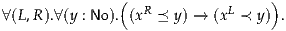 | (11.6.10) |
We now have to define (x ≺ y) and (x ≼ y) for all y. Here in contrast
to Theorem 11.3.16, rather than a nested recursion, we use a nested
induction, in order to be able to inductively use transitivity on the left with
respect to the inequalities xL < x and x < xR. Define A′ : No → by
taking A′(y) to be the subset A′ of Prop ×Prop consisting of two mere
propositions, denoted △≼ y and △≺ y (with △ : A′(y)), such that
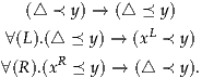 | (11.6.11) (11.6.12) (11.6.13) |
| (△⊑□) | :≡ (△≼ y) → (□≼ z) (△≼ y) → (□≼ z) ∧ ∧ (△≺ y) → (□≺ z) (△≺ y) → (□≺ z) | ||
| (△⊏ □) | :≡ (△≼ y) → (□≺ z) (△≼ y) → (□≺ z) . . |
For the primary clause of the inner induction, we assume also given y defined by a cut, and properties (x ≺ yL), (x ≺ yR), (x ≼ yL), and (x ≼ yR) for all L and R, with the strict ones implying the non-strict ones, transitivity on the left with respect to xL < x and x < xR, and on the right with respect to yL < yR. We can now give the definitions specified in the theorem statement:
| (x ≼ y) | :≡ (∀(L).xL ≺ y) ∧ (∀(R).x ≺ yR), | (11.6.14) |
| (x ≺ y) | :≡ (∃(L).x ≼ yL) ∨ (∃(R).xR ≼ y). | (11.6.15) |
On the other hand, if there is R0 with xR0 ≼ y, then by transitivity on the left with respect to xL < xR0 we have xL ≺ y for all L. And by transitivity on the left and right with respect to x < xR0 and y < yR, we have x ≺ yR for any R. Thus, x ≼ y.
We also need to show that these definitions are transitive on the left with respect to xL < x and x < xR. But if x ≼ y, then xL ≺ y for all L by definition; while if xR ≼ y, then x ≺ y also by definition.
Thus, (11.6.14) and (11.6.15) do define an element of A′(y). We now have to verify that this definition preserves inequalities, as a dependent function into A′, i.e. that these relations are transitive on the right. Remember that in each case, we may assume inductively that they are transitive on the right with respect to all inequalities arising in the inequality constructor.
Second, suppose y < z arises from yR0 ≤ z. Then by definition, x ≼ y implies x ≺ yR0, and then the inner inductive hypothesis for yR0 ≤ z yields x ≺ z.
This completes the inner induction. Thus, for any x defined by a cut, we have (x ≺ –) and (x ≼ –) defined by (11.6.14) and (11.6.15), and transitive on the right.
To complete the outer recursion, we need to verify these definitions are transitive on the left. After a No-induction on z, we end up with three cases that are essentially identical to those just described above for transitivity on the right. Hence, we omit them. __
Proof. From left to right, we use (No, ≤, <)-induction where A(x) :≡1, with ≼ and ≺ supplying the relations ⊴ and ◃. In all the constructor cases, x and y are defined by cuts, so the definitions of ≼ and ≺ evaluate, and the inductive hypotheses apply.
From right to left, we use No-induction to assume that x and y are defined by cuts. But now the definitions of ≼ and ≺, and the inductive hypotheses, supply exactly the data required for the relevant constructors of ≤ and <. __
As with the Cauchy reals, the joint (No, ≤, <)-recursion principle remains essential when defining all operations on No.
Example 11.6.18. We define + : No →No →No by a double recursion. For the outer recursion, we take the codomain to be the subset of No →No consisting of functions g such that (x < y) → (g(x) < g(x)) and (x ≤ y) → (g(x) ≤ g(y)) for all x, y. For such g, h we define (g ⊴ h) :≡∀(x : No).g(x) ≤ h(x) and (g ◃ h) :≡∀(x : No).g(x) < h(x). Clearly ⊴ is antisymmetric.
For the primary clause of the recursion, we suppose x defined by a cut, and we define (x + –) by an inner recursion on No with codomain No, with relations ⊑ and ⊏ coinciding with ≤ and <. For the primary clause of the inner recursion, we suppose also y defined by a cut, and give Conway’s definition:

In other words, the left options of x + y are all numbers of the form xL + y for some left option xL, or x + yL for some left option yL. Now we verify that this definition preserves inequality:
This completes the inner recursion. For the outer recursion, we have to verify that + preserves inequality on the left as well. After an No-induction, this proceeds in exactly the same way.
In the Appendix to Part Zero of [Con76], Conway discusses how the surreal numbers may be formalized in ZFC set theory: by iterating along the ordinals and passing to sets of representatives of lowest rank for each equivalence class, or by representing numbers with “sign-expansions”. He then remarks that
The curiously complicated nature of these constructions tells us more about the nature of formalizations within ZF than about our system of numbers…
and goes on to advocate for a general theory of “permissible kinds of construction” which should include
Condition (i) can be naturally read as justifying general principles of inductive definition, such as those presented in §§5.6 and 5.7. In particular, the condition of strict positivity for constructors can be regarded as a formalization of what it means to be “reasonably constructive”. Condition (ii) then suggests we should extend this to higher inductive definitions of all sorts, in which we can impose path constructors making objects equal in any reasonable way. For instance, in the next paragraph Conway says:
…we could also, for instance, freely create a new object (x, y) and call it the ordered pair of x and y. We could also create an ordered pair [x, y] different from (x, y) but co-existing with it…If instead we wanted to make (x, y) into an unordered pair, we could define equality by means of the equivalence relation (x, y) = (z, t) if and only if x = z, y = t or x = t, y = z.
The freedom to introduce new objects with new names, generated by certain forms of constructors, is precisely what we have in the theory of inductive definitions. Just as with our two copies of the natural numbers N and N′ in §5.2, if we wrote down an identical definition to the cartesian product type A×B, we would obtain a distinct product type A×′B whose canonical elements we could freely write as [x, y]. And we could make one of these a type of unordered pairs by adding a suitable path constructor.
To be sure, Conway’s point was not to complain about ZF in particular, but to argue against all foundational theories at once:
…this proposal is not of any particular theory as an alternative to ZF… What is proposed is instead that we give ourselves the freedom to create arbitrary mathematical theories of these kinds, but prove a metatheorem which ensures once and for all that any such theory could be formalized in terms of any of the standard foundational theories.
One might respond that, in fact, univalent foundations is not one of the “standard foundational theories” which Conway had in mind, but rather the metatheory in which we may express our ability to create new theories, and about which we may prove Conway’s metatheorem. For instance, the surreal numbers are one of the “mathematical theories” Conway has in mind, and we have seen that they can be constructed and justified inside univalent foundations. Similarly, Conway remarked earlier that
…set theory would be such a theory, sets being constructed from earlier ones by processes corresponding to the usual axioms, and the equality relation being that of having the same members.
This description closely matches the higher-inductive construction of the cumulative hierarchy of set theory in §10.5. Conway’s metatheorem would then correspond to the fact we have referred to several times that we can construct a model of univalent foundations inside ZFC (which is outside the scope of this book).
However, univalent foundations is so rich and powerful in its own right that it would be foolish to relegate it to only a metatheory in which to construct set-like theories. We have seen that even at the level of sets (0-types), the higher inductive types in univalent foundations yield direct constructions of objects by their universal properties (§6.11), such as a constructive theory of Cauchy completion (§11.3). But most importantly, the potential to model homotopy theory and category theory directly in the foundational system (Chapters 8 and 9) gives univalent foundations an advantage which no set-theoretic foundation can match.
Defining algebraic operations on Dedekind reals, especially multiplication, is both somewhat tricky and tedious. There are several ways to get arithmetic going: each has its own advantages, but they all seem to require some technical work. For instance, Richman [Ric08] defines multiplication on the Dedekind reals first on the positive cuts and then extends it algebraically to all Dedekind cuts, while Conway [Con76] has observed that the definition of multiplication for surreal numbers works well for Dedekind reals.
Our treatment of the Dedekind reals borrows many ideas from [BT09] where the Dedekind reals are constructed in the context of Abstract Stone Duality. This is a (restricted) form of simply typed λ-calculus with a distinguished object Σ which classifies open sets, and by duality also the closed ones. In [BT09] you can also find detailed proofs of the basic properties of arithmetical operations.
The fact that Rc is the least Cauchy complete archimedean ordered field, as was proved in Theorem 11.3.50, indicates that our Cauchy reals probably coincide with the Escardó-Simpson reals [ES01]. It would be interesting to check whether this is really the case. The notion of Escardó-Simpson reals, or more precisely the corresponding closed interval, is interesting because it can be stated in any category with finite products.
In constructive set theory augmented by the “regular extension axiom”, one may also try to define Cauchy completion by closing under limits of Cauchy sequences with a transfinite iteration. It would also be interesting to check whether this construction agrees with ours.
It is constructive folklore that coincidence of Cauchy and Dedekind reals requires dependent choice but it is less well known that countable choice suffices. Recall that dependent choice states that for a total relation R on A, by which we mean ∀(x : A).∃(y : A).R(x, y), and for any a : A there merely exists f : N → A such that f(0) = a and R(f(n), f(n + 1)) for all n : N. Our Corollary 11.4.3 uses the typical trick for converting an application of dependent choice to one using countable choice. Namely, we use countable choice once to make in advance all the choices that could come up, and then use the choice function to avoid the dependent choices.
The intricate relationship between various notions of compactness in a constructive setting is discussed in [BIS02]. Palmgren [Pal07] has a good comparison between pointwise analysis and pointfree topology.
The surreal numbers were defined by [Con76], using a sort of inductive definition but without justifying it explicitly in terms of any foundational system. For this reason, some later authors have tended to use sign-expansions or other more explicit presentations which can be coded more obviously into set theory. The idea of representing them in type theory was first considered by Hancock, while Setzer and Forsberg [FS12] noted that the surreals and their inequality relations < and ≤ naturally form an inductive-inductive definition. The higher inductive-inductive version presented here, which builds in the correct notion of equality for surreals, is new.
Exercise 11.1. Give an alternative definition of the Dedekind reals by first defining the square and then use Eq. (11.3.45). Check that one obtains a commutative ring.
Exercise 11.2. Suppose we remove the boundedness condition in Definition 11.2.1. Then we obtain the extended reals which contain -∞ :≡ (0, Q) and ∞ :≡ (Q, 0). Which definitions of arithmetical operations on cuts still make sense for extended reals? What algebraic structure do we get?
Exercise 11.3. By considering one-sided cuts we obtain lower and upper Dedekind reals, respectively. For example, a lower real is given by a predicate L : Q → Ω which is
(We could also require ∃(r : Q).¬L(r) to exclude the cut ∞:≡Q.) Which arithmetical operations can you define on the lower reals? In particular, what happens with the additive inverse?
Exercise 11.4. Suppose we remove the locatedness condition in Definition 11.2.1. Then we obtain the interval domain I because cuts are allowed to have “gaps”, which are just intervals. Define the partial order ⊑ on I by
 " class="math-display" >
Exercise 11.7. Show that in an ordered field F, density of Q and the traditional archimedean axiom are equivalent:
 |
Exercise 11.8. Suppose a, b : Q and f :  a ≤ q ≤ b} → Rc is
Lipschitz with constant L. Show that there exists a unique extension
: [a, b] → Rc of f which is Lipschitz with constant L. Hint: rather
than redoing Lemma 11.3.15 for closed intervals, observe that there is a
retraction r : Rc → [-n, n] and apply Lemma 11.3.15 to f ∘r.
a ≤ q ≤ b} → Rc is
Lipschitz with constant L. Show that there exists a unique extension
: [a, b] → Rc of f which is Lipschitz with constant L. Hint: rather
than redoing Lemma 11.3.15 for closed intervals, observe that there is a
retraction r : Rc → [-n, n] and apply Lemma 11.3.15 to f ∘r.
Exercise 11.9. Generalize the construction of Rc to construct the Cauchy completion of any metric space. First, think about which notion of real numbers is most natural as the codomain for the distance function of a metric space. Does it matter? Next, work out the details of two constructions:
The idea is that f looks like it is measuring the distance from a point.
Finally, prove the following universal property of metric completions: a locally uniformly continuous map from a metric space to a Cauchy complete metric space extends uniquely to a locally uniformly continuous map on the completion. (We say that a map is locally uniformly continuous if it is uniformly continuous on open balls.)
Exercise 11.10. Markov’s principle says that for all f : N →2,
 |
This is a particular instance of the law of double negation (3.4.2). Show that ∀(x, y : Rd).x≠y ⇒ x # y implies Markov’s principle. Does the converse hold as well?
Exercise 11.11. Verify that the following “no zero divisors” property holds for the real numbers: xy # 0 ⇔ x # 0 ∧y # 0.
Exercise 11.12. Suppose (q1, r1), …, (qn, rn) pointwise cover (a, b). Then there is ϵ : Q+ such that whenever a < x < y < b and |x-y| < ϵ then there merely exists i such that qi < x < ri and qi < y < ri. Such an ϵ is called a Lebesgue number for the given cover.
Exercise 11.13. Prove the following approximate version of the intermediate value theorem:
If f : [0, 1] →R is uniformly continuous and f(0) < 0 < f(1) then for every ϵ : Q+ there merely exists x : [0, 1] such that |f(x)| < ϵ.
Hint: do not try to use the bisection method because it leads to the axiom of choice. Instead, approximate f with a piecewise linear map. How do you construct a piecewise linear map?
Exercise 11.14. Check whether everything in [Knu74] can be done using the higher inductive-inductive surreals of §11.6.
Just as one can develop mathematics in set theory without explicitly using the axioms of Zermelo–Fraenkel set theory, in this book we have developed mathematics in univalent foundations without explicitly referring to a formal system of homotopy type theory. Nevertheless, it is important to have a precise description of homotopy type theory as a formal system in order to, for example,
Even the logical consistency of homotopy type theory, namely that in the empty context there is no term a : 0, is not obvious: if we had erroneously chosen a definition of equivalence for which 0 ≃1, then univalence would imply that 0 has an element, since 1 does. Nor is it obvious that, for example, our definition of S1 as a higher inductive type yields a type which behaves like the ordinary circle.
There are two aspects of type theory which we must pin down before addressing such questions. Recall from the Introduction that type theory comprises a set of rules specifying when the judgments a : A and a ≡ a′ : A hold—for example, products are characterized by the rule that whenever a : A and b : B, (a, b) : A×B. To make this precise, we must first define precisely the syntax of terms—the objects a, a′, A, … which these judgments relate; then, we must define precisely the judgments and their rules of inference—the manner in which judgments can be derived from other judgments.
In this appendix, we present two formulations of Martin-Löf type theory, and of the extensions that constitute homotopy type theory. The first presentation (Appendix A.1) describes the syntax of terms and the forms of judgments as an extension of the untyped λ-calculus, while leaving the rules of inference informal. The second (Appendix A.2) defines the terms, judgments, and rules of inference inductively in the style of natural deduction, as is customary in much type-theoretic literature.
In Chapter 1, we presented the two basic judgments of type theory. The first, a : A, asserts that a term a has type A. The second, a ≡ b : A, states that the two terms a and b are judgmentally equal at type A. These judgments are inductively defined by a set of inference rules described in Appendix A.2.
To construct an element a of a type A is to derive a : A; in the book, we give informal arguments which describe the construction of a, but formally, one must specify a precise term a and a full derivation that a : A.
However, the main difference between the presentation of type theory in the book and in this appendix is that here judgments are explicitly formulated in an ambient context, or list of assumptions, of the form

An element xi : Ai of the context expresses the assumption that the variable xi has type Ai. The variables x1, …, xn appearing in the context must be distinct. We abbreviate contexts with the letters Γ and Δ.
The judgment a : A in context Γ is written

and means that a : A under the assumptions listed in Γ. When the list of assumptions is empty, we write simply

or

where ⋅ denotes the empty context. The same applies to the equality judgment

However, such judgments are sensible only for well-formed contexts, a notion captured by our third and final judgment

expressing that each Ai is a type in the context x1 : A1, x2 : A2, …, xi-1 : Ai-1. In particular, therefore, if Γ ⊢ a : A and Γ ctx, then we know that each Ai contains only the variables x1, …, xi-1, and that a and A contain only the variables x1, …, xn.
In informal mathematical presentations, the context is implicit. At each point in a proof, the mathematician knows which variables are available and what types they have, either by historical convention (n is usually a number, f is a function, etc.) or because variables are explicitly introduced with sentences such as “let x be a real number”. We discuss some benefits of using explicit contexts in Appendices A.2.4 and A.2.5.
We write B[a/x] for the substitution of a term a for free occurrences of the variable x in the term B, with possible capture-avoiding renaming of bound variables, as discussed in §1.2. The general form of substitution
![B [a1,...,an/x1,...,xn]](hott-html4452x.png)
substitutes expressions a1, …, an for the variables x1, …, xn simultaneously.
To bind a variable xin an expression B means to incorporate both of them
into a larger expression, called an abstraction, whose purpose is to express the
fact that x is “local” to B, i.e., it is not to be confused with other occurrences of
x appearing elsewhere. Bound variables are familiar to programmers, but less
so to mathematicians. Various notations are used for binding, such as x B,
λx.B, and x.B, depending on the situation. We may write C[a] for the
substitution of a term a for the variable in the abstracted expression, i.e., we
may define (x.B)[a] to be B[a/x]. As discussed in §1.2, changing the name of a
bound variable everywhere within an expression (“α-conversion”) does not
change the expression. Thus, to be very precise, an expression is an
equivalence class of syntactic forms which differ in names of bound
variables.
B,
λx.B, and x.B, depending on the situation. We may write C[a] for the
substitution of a term a for the variable in the abstracted expression, i.e., we
may define (x.B)[a] to be B[a/x]. As discussed in §1.2, changing the name of a
bound variable everywhere within an expression (“α-conversion”) does not
change the expression. Thus, to be very precise, an expression is an
equivalence class of syntactic forms which differ in names of bound
variables.
One may also regard each variable xi of a judgment

to be bound in its scope, consisting of the expressions Ai+1, …, An, a, and A.
The objects and types of our type theory may be written as terms using the following syntax, which is an extension of λ-calculus with variables x, x′, …, primitive constants c, c′, …, defined constants f, f′, …, and term forming operations
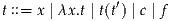
The notation used here means that a term t is either a variable x, or it has the form λx.t where x is a variable and t is a term, or it has the form t(t′) where t and t′ are terms, or it is a primitive constant c, or it is a defined constant f. The syntactic markers ’λ’, ’(’, ’)’, and ’.’ are punctuation for guiding the human eye.
We use t(t1, …, tn) as an abbreviation for the repeated application t(t1)(t2)…(tn). We may also use infix notation, writing t1 ⋆t2 for ⋆(t1, t2) when ⋆ is a primitive or defined constant.
Each defined constant has zero, one or more defining equations. There are two kinds of defined constant. An explicit defined constant f has a single defining equation
where t does not involve f. For example, we might introduce the explicit defined constant ∘ with defining equation
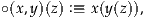
and use infix notation x∘y for ∘(x, y). This of course is just composition of functions.
The second kind of defined constant is used to specify a (parameterized) mapping f(x1, …, xn, x), where x ranges over a type whose elements are generated by zero or more primitive constants. For each such primitive constant c there is a defining equation of the form

where f may occur in t, but only in such a way that it is clear that the equations determine a totally defined function. The paradigm examples of such defined functions are the functions defined by primitive recursion on the natural numbers. We may call this kind of definition of a function a total recursive definition. In computer science and logic this kind of definition of a function on a recursive data type has been called a definition by structural recursion.
Convertibility t ↓ t′ between terms t and t′ is the equivalence relation generated by the defining equations for constants, the computation rule
![(λx .t)(u) :≡ t[u/x],](hott-html4463x.png)
and the rules which make it a congruence with respect to application and λ-abstraction:
The equality judgment t ≡ u : A is then derived by the following single rule:
Judgmental equality is an equivalence relation.
We postulate a hierarchy of universes denoted by primitive constants
 |
The first two rules for universes say that they form a cumulative hierarchy of types:
m : n for m < n,
m and m ≤ n, then A : n,and the third expresses the idea that an object of a universe can serve as a type and stand to the right of a colon in judgments:
n, and x is a new variable,1
then ⊢ (Γ, x : A)ctx.In the body of the book, an equality judgment A ≡ B : n between types A and B
is usually abbreviated to A ≡ B. This is an instance of typical ambiguity, as
we can always switch to a larger universe, which however does not affect the
validity of the judgment.
The following conversion rule allows us to replace a type by one equal to it in a typing judgment:
We introduce a primitive constant cΠ, but write cΠ(A, λx.B) as ∏(x:A) B. Judgments concerning such expressions and expressions of the form λx.b are introduced by the following rules:
n and Γ, x : A ⊢ B : n, then Γ ⊢ ∏(x:A) B : n
If x does not occur freely in B, we abbreviate ∏(x:A) B as the non-dependent function type A → B and derive the following rule:
Using non-dependent function types and leaving implicit the context Γ, the rules above can be written in the following alternative style that we use in the rest of this section of the appendix.
n and B : A →n, then ∏(x:A) B(x) : n
We introduce primitive constants cΣ and cpair. An expression of the form cΣ(A, λa.B) is written as ∑(a:A) B, and an expression of the form cpair(a, b) is written as (a, b). We write A×B instead of ∑(x:A) B if x is not free in B.
Judgments concerning such expressions are introduced by the following rules:
n and B : A →n, then ∑(x:A) B(x) : n
If we have A and B as above, C : ∑(x:A) B(x) →m, and
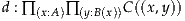
we can introduce a defined constant
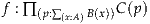
with the defining equation
Note that C, d, x, and y may contain extra implicit parameters x1, …, xn if they were obtained in some non-empty context; therefore, the fully explicit recursion schema is

We introduce primitive constants c+, cinl, and cinr. We write A + B instead of c+(A, B), inl(a) instead of cinl(a), and inr(a) instead of cinr(a):
n then A + B : n
If we have A and B as above, C : A + B →m, d : ∏(x:A) C(inl(x)), and
e : ∏(y:B) C(inr(y)), then we can introduce a defined constant f : ∏(z:A+B) C(z)
with the defining equations
 |
We introduce primitive constants ⋆, 0, 1, satisfying the following rules:
0, 1 : 0
Given C : 0 →n we can introduce a defined constant f : ∏(x:0) C(x),
with no defining equations.
Given C : 1 →n and d : C(⋆) we can introduce a defined constant
f : ∏(x:1) C(x), with defining equation f(⋆) :≡ d.
The type of natural numbers is obtained by introducing primitive constants N, 0, and succ with the following rules:
0,
Furthermore, we can define functions by primitive recursion. If we have
C : N →k we can introduce a defined constant f : ∏(x:N) C(x) whenever
we have
| d | : C(0) | ||
| e | : ∏(x:N)(C(x) → C(succ(x))) |
 |
For W-types we introduce primitive constants cW and csup. An expression of the form cW(A, λx.B) is written as W(x:A)B, and an expression of the form csup(x, u) is written as sup(x, u):
n and B : A →n, then W(x:A)B(x) : n
Here also we can define functions by total recursion. If we have A and B as above
and C : W(x:A)B(x) →m, then we can introduce a defined constant
f : ∏(z:W(x:A)B(x)) C(z) whenever we have

with the defining equation
We introduce primitive constants c= and crefl. We write a =A b for c=(A, a, b) and refla for crefl(A, a), when a : A is understood:
n, a : A, and b : A then a =A b : n.
Given a : A, if y : A, z : a =A y ⊢ C : m and ⊢ d : C[a, refla/y, z] then we can
introduce a defined constant
with defining equation
In this section, there are three kinds of judgments

 |
It says that we may derive the conclusion  , provided that we have already
derived the hypotheses 1, …, k. (Note that, being judgments rather than
types, these are not hypotheses internal to the type theory in the sense of
§1.1; they are instead hypotheses in the deductive system, i.e. the
metatheory.) On the right we write the Name of the rule, and there
may be extra side conditions that need to be checked before the rule is
applicable.
, provided that we have already
derived the hypotheses 1, …, k. (Note that, being judgments rather than
types, these are not hypotheses internal to the type theory in the sense of
§1.1; they are instead hypotheses in the deductive system, i.e. the
metatheory.) On the right we write the Name of the rule, and there
may be extra side conditions that need to be checked before the rule is
applicable.
A derivation of a judgment is a tree constructed from such inference rules, with the judgment at the root of the tree. For example, with the rules given below, the following is a derivation of ⋅⊢ λx.x : 1 →1.
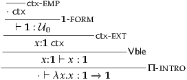
A context is a list
 |
which indicates that the distinct variables x1, …, xn are assumed to have types A1, …, An, respectively. The list may be empty. We abbreviate contexts with the letters Γ and Δ, and we may juxtapose them to form larger contexts.
The judgment Γ ctx formally expresses the fact that Γ is a well-formed context, and is governed by the rules of inference
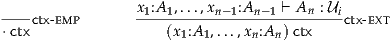 i; while the conclusion
says that the extended context (x1:A1, …, xn:An) is well-formed. (It is a
meta-theoretic property of the system that if x1:A1, …, xn:An ⊢ b : B is
derivable, then the context (x1:A1, …, xn:An) must be well-formed; thus
ctx-ext does not need to hypothesize well-formedness of the context to the
left of xn.)
i; while the conclusion
says that the extended context (x1:A1, …, xn:An) is well-formed. (It is a
meta-theoretic property of the system that if x1:A1, …, xn:An ⊢ b : B is
derivable, then the context (x1:A1, …, xn:An) must be well-formed; thus
ctx-ext does not need to hypothesize well-formedness of the context to the
left of xn.)
The fact that the context holds assumptions is expressed by the rule which says that we may derive those typing judgments which are listed in the context:
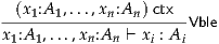
The following important principles, called substitution and weakening, need not be explicitly assumed. Rather, it is possible to show, by induction on the structure of all possible derivations, that whenever the hypotheses of these rules are derivable, their conclusion is also derivable.2 For the typing judgments these principles are manifested as
![Γ-⊢-a : A---Γ ,x-:A-,Δ-⊢-b :-BSubst Γ-⊢ A-: Ui--Γ ,Δ-⊢-b : B-Wkg
Γ ,Δ [a/x] ⊢ b[a/x] : B[a/x] 1 Γ ,x:A,Δ ⊢ b : B 1](hott-html4501x.png)
![--Γ ⊢-a :-A--Γ ,x:A-,Δ-⊢ b-≡-c : B-Subst2
Γ ,Δ [a/x] ⊢ b[a/x] ≡ c[a/x] : B[a/x]
Γ-⊢-A-: Ui---Γ ,Δ-⊢-b-≡-c : B
Γ ,x :A ,Δ ⊢ b ≡ c : B Wkg2](hott-html4502x.png)
Γ ⊢ a : A__
Γ ⊢ a ≡ a : A Γ ⊢ a ≡ b : A___________
Γ ⊢ b ≡ a : A Γ ⊢ a ≡ b : A Γ ⊢ b ≡ c : A__________________________
Γ ⊢ a ≡ c : A
Γ ⊢ a : A Γ ⊢ A ≡ B : i
________________________
Γ ⊢ a : B Γ ⊢ a ≡ b : A Γ ⊢ A ≡ B : i___________________________
Γ ⊢ a ≡ b : B
Additionally, for all the type formers below, we assume rules stating that each constructor preserves definitional equality in each of its arguments; for instance, along with the Π-intro rule, we assume the rule
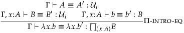
However, we omit these rules for brevity.
We postulate an infinite hierarchy of type universes
 |
Each universe is contained in the next, and any type in i is also in
i+1:
 i for some i. In other words, if A plays the role of a type then it is in
some universe. Another property of our type system is that Γ ⊢ a ≡ b : A
implies Γ ⊢ a : A and Γ ⊢ b : A.
i for some i. In other words, if A plays the role of a type then it is in
some universe. Another property of our type system is that Γ ⊢ a ≡ b : A
implies Γ ⊢ a : A and Γ ⊢ b : A.
In §1.2, we introduced non-dependent functions A → B in order to define a
family of types as a function λ(x:A).B : A →i, which then gives rise to a
type of dependent functions ∏(x:A) B. But with explicit contexts we may
replace λ(x:A).B : A →i with the judgment
 |
Consequently, we may define dependent functions directly, without reference to non-dependent ones. This way we follow the general principle that each type former, with its constants and rules, should be introduced independently of all other type formers. In fact, henceforth each type former is introduced systematically by:
(See also Remark 1.5.1.)
For the dependent function type these rules are:
Γ ⊢ A : i Γ, x:A ⊢ B : i_________________________
Γ ⊢∏(x:A)B : i
Π-form
Γ, x:A ⊢ b : B
____
Γ ⊢ λ(x:A).b : ∏(x:A)BΠ-intro Γ ⊢ f : ∏(x:A)B Γ ⊢ a : A
________________________
Γ ⊢ f(a) : B[a/x]
Π-elim
Γ, x:A ⊢ b : B Γ ⊢ a : A
____
Γ ⊢ (λ(x:A).b)(a) ≡ b[a/x] : B[a/x]Π-comp
Γ ⊢ f : ∏(x:A)B
_____
Γ ⊢ f ≡ (λx.f(x)) : ∏(x:A)BΠ-uniq
The expression λ(x:A).b binds free occurrences of x in b, as does ∏(x:A) B for B.
When x does not occur freely in B so that B does not depend on A, we obtain as a special case the ordinary function type A → B :≡ ∏(x:A) B. We take this as the definition of →.
We may abbreviate an expression λ(x:A).b as λx.b, with the understanding that the omitted type A should be filled in appropriately before type-checking.
In §1.6, we needed → and ∏ types in order to define the introduction and elimination rules for ∑; as with ∏, contexts allow us to state the rules for ∑ independently. Recall that the elimination rule for a positive type such as Σ is called induction and denoted by ind.
Γ ⊢ A : i Γ, x:A ⊢ B : i_________________________
Γ ⊢∑(x:A)B : i
Σ-form
Γ, x:A ⊢ B : i Γ ⊢ a : A Γ ⊢ b : B[a/x]
_______________________________________
Γ ⊢ (a, b) : ∑(x:A)B
Σ-intro
Γ, z:∑(x:A)B ⊢ C : i
Γ, x:A, y:B ⊢ g : C[(x, y)/z] Γ ⊢ p : ∑(x:A)B
Γ ⊢ind∑(x:A) B(z.C, x.y.g, p) : C[p/z]
Σ-elim
Γ, z:∑(x:A)B ⊢ C : i Γ, x:A, y:B ⊢ g : C[(x, y)/z]
Γ ⊢ a′ : A Γ ⊢ b′ : B[a′/x]
_____________
Γ ⊢ind∑(x:A) B(z.C, x.y.g, (a′, b′)) ≡ g[a′, b′/x, y] : C[(a′, b′)/z]Σ-comp
The expression ∑(x:A) B binds free occurrences of x in B. Furthermore, because ind∑(x:A) B has some arguments with free variables beyond those in Γ, we bind (following the variable names above) z in C, and x and y in g. These bindings are written as z.C and x.y.g, to indicate the names of the bound variables. In particular, we treat ind∑(x:A) B as a primitive, two of whose arguments contain binders; this is superficially similar to, but different from, ind∑(x:A) B being a function that takes functions as arguments.
When B does not contain free occurrences of x, we obtain as a special case the cartesian product A×B :≡ ∑(x:A) B. We take this as the definition of the cartesian product.
Notice that we don’t postulate a judgmental uniqueness principle for Σ-types, even though we could have; see Corollary 2.7.3 for a proof of the corresponding propositional uniqueness principle.
Γ ⊢ A : i Γ ⊢ B : i_____________________
Γ ⊢ A + B : i
+-form
Γ ⊢ A : i Γ ⊢ B : i
Γ ⊢ a : A
_______
Γ ⊢inl(a) : A + B
+-intro1
Γ ⊢ A : i Γ ⊢ B : i
Γ ⊢ b : B
_______
Γ ⊢inr(b) : A + B
+-intro2
Γ, z:(A + B) ⊢ C : i
Γ, x:A ⊢ c : C[inl(x)/z] Γ, y:B ⊢ d : C[inr(y)/z]
Γ ⊢ e : A + B
_______________
Γ ⊢indA+B(z.C, x.c, y.d, e) : C[e/z]
+-elim
Γ, z:(A + B) ⊢ C : i
Γ, x:A ⊢ c : C[inl(x)/z] Γ, y:B ⊢ d : C[inr(y)/z]
Γ ⊢ a : A
__________________
Γ ⊢indA+B(z.C, x.c, y.d, inl(a)) ≡ c[a/x] : C[inl(a)/z]+-comp1
Γ, z:(A + B) ⊢ C : i
Γ, x:A ⊢ c : C[inl(x)/z] Γ, y:B ⊢ d : C[inr(y)/z]
Γ ⊢ b : B
___________________
Γ ⊢indA+B(z.C, x.c, y.d, inr(b)) ≡ d[b/y] : C[inr(b)/z]+-comp2
In indA+B, z is bound in C, x is bound in c, and y is bound in d.
Γ ctx__
Γ ⊢0 : i
0-form Γ, x:0 ⊢ C : i Γ ⊢ a : 0______________________
Γ ⊢ind0(x.C, a) : C[a/x] 0-elim
In ind0, x is bound in C. The empty type has no introduction rule and no computation rule.
Γ ctx__
Γ ⊢1 : i
1-form Γ ctx_
Γ ⊢ ⋆ : 11-intro
Γ, x:1 ⊢ C : i Γ ⊢ c : C[⋆/x] Γ ⊢ a : 1
______________________________________
Γ ⊢ind1(x.C, c, a) : C[a/x]
1-elim
Γ, x:1 ⊢ C : i Γ ⊢ c : C[⋆/x]
___________________________
Γ ⊢ind1(x.C, c, ⋆) ≡ c : C[⋆/x]
1-comp
In ind1 the variable x is bound in C.
Notice that we do not postulate a judgmental uniqueness principle for the unit type; see §1.5 for a proof of the corresponding propositional uniqueness statement.
We give the rules for natural numbers, following §1.9.
Γ ctx__
Γ ⊢N : i
N-form Γ ctx__
Γ ⊢ 0 : NN-intro1 Γ ⊢ n : N___
Γ ⊢succ(n) : NN-intro2
Γ, x:N ⊢ C : i
Γ ⊢ c0 : C[0/x] Γ, x:N, y:C ⊢ cs : C[succ(x)/x] Γ ⊢ n : N
_____________________________________________________
Γ ⊢indN(x.C, c0, x.y.cs, n) : C[n/x]
N-elim
Γ, x:N ⊢ C : i
Γ ⊢ c0 : C[0/x] Γ, x:N, y:C ⊢ cs : C[succ(x)/x]
_________________________________________
Γ ⊢indN(x.C, c0, x.y.cs, 0) ≡ c0 : C[0/x]
N-comp1
Γ, x:N ⊢ C : i Γ ⊢ c0 : C[0/x]
Γ, x:N, y:C ⊢ cs : C[succ(x)/x] Γ ⊢ n : N
_____________________________________
Γ ⊢indN(x.C, c0, x.y.cs, succ(n))
≡ cs[n, indN(x.C, c0, x.y.cs, n)/x, y] : C[succ(n)/x]N-comp2
In indN, x is bound in C, and x and y are bound in cs.
Other inductively defined types follow the same general scheme.
The presentation here corresponds to the (unbased) path induction principle for identity types in §1.12.
Γ ⊢ A : i Γ ⊢ a : A Γ ⊢ b : A_______________________________
Γ ⊢ a =A b : i
=
-form
Γ ⊢ A : i Γ ⊢ a : A
____________________
Γ ⊢refla : a =A a
=
-intro
Γ, x:A, y:A, p:x =A y ⊢ C : i Γ, z:A ⊢ c : C[z, z, reflz/x, y, p]
Γ ⊢ a : A Γ ⊢ b : A Γ ⊢ p′ : a =A b
_________
Γ ⊢ind=A(x.y.p.C, z.c, a, b, p′) : C[a, b, p′/x, y, p]
=
-elim
Γ, x:A, y:A, p:x =A y ⊢ C : i
Γ, z:A ⊢ c : C[z, z, reflz/x, y, p] Γ ⊢ a : A
_______
Γ ⊢ind=A(x.y.p.C, z.c, a, a, refla) ≡ c[a/z] : C[a, a, refla/x, y, p]=-comp
In ind=A, x, y, and p are bound in C, and z is bound in c.
Although the rules we listed so far allows us to construct everything we need directly, we would still like to be able to use named constants, such as isequiv, as a matter of convenience. Informally, we can think of these constants simply as abbreviations, but the situation is a bit subtler in the formalization.
For example, consider function composition, which takes f : A → B and g : B → C to g∘f : A → C. Somewhat unexpectedly, to make this work formally, ∘ must take as arguments not only f and g, but also their types A, B, C:

Inference of implicit arguments, typical ambiguity (§1.3), ensuring that symbols are only defined once, etc., are collectively called elaboration. Elaboration must take place prior to checking a derivation, and is thus not usually presented as part of the core type theory. However, it is essentially impossible to use any implementation of type theory which does not perform elaboration; see [Coq12, Nor07] for further discussion.
In this section we state the additional axioms of homotopy type theory which distinguish it from standard Martin-Löf type theory: function extensionality, the univalence axiom, and higher inductive types. We state them in the style of the second presentation Appendix A.2, although the first presentation Appendix A.1 could be used just as well.
There are two basic ways of introducing axioms which do not introduce new syntax or judgmental equalities (function extensionality and univalence are of this form): either add a primitive constant to inhabit the axiom, or prove all theorems which depend on the axiom by hypothesizing a variable that inhabits the axiom, cf. §1.1. While these are essentially equivalent, we opt for the former approach because we feel that the axioms of homotopy type theory are an essential part of the core theory.
Axiom 2.9.3 is formalized by introduction of a constant funext which asserts that happly is an equivalence:
Γ ⊢ f : ∏(x:A)B Γ ⊢ g : ∏(x:A)B Γ ⊢funext(f, g) : isequiv(happlyf,g) Π-ext
The definitions of happly and isequiv can be found in (2.9.2) and §4.5, respectively.
Axiom 2.10.3 is formalized in a similar fashion, too:
Γ ⊢ A : i Γ ⊢ B : i_______
Γ ⊢univalence(A, B) : isequiv(idtoeqvA,B) i-univ
The definition of idtoeqv can be found in (2.10.2).
Here we give an example of a basic higher inductive type; others follow the same general scheme, albeit with elaborations.
Note that the rules below do not precisely follow the pattern of the ordinary inductive types in Appendix A.2: the rules refer to the notions of transport and functoriality of maps (§2.2), and the second computation rule is a propositional, not judgmental, equality. These differences are discussed in §6.2.
Γ ctx__
Γ ⊢S1 : i
S1-form Γ ctx___
Γ ⊢base : S1
S1-intro1
Γ ctx
_______
Γ ⊢loop : base =S1 baseS1-intro2
Γ, x:S1 ⊢ C : i
Γ ⊢ b : C[base/x] Γ ⊢ ℓ : b =Cloop b Γ ⊢ p : S1
___________________________________________
Γ ⊢indS1(x.C, b, ℓ, p) : C[p/x]
S1-elim
Γ, x:S1 ⊢ C : i Γ ⊢ b : C[base/x] Γ ⊢ ℓ : b =Cloop b
Γ ⊢indS1(x.C, b, ℓ, base) ≡ b : C[base/x] S1-comp1
Γ, x:S1 ⊢ C : i Γ ⊢ b : C[base/x] Γ ⊢ ℓ : b =Cloop b
Γ ⊢S1-loopcomp : apd(λy.ind
S1(x.C,b,ℓ,y)) = ℓ
S1-comp2
= ℓ
S1-comp2
In indS1, x is bound in C. The notation b =Cloop b for dependent paths was introduced in §6.2.
This section discusses the meta-theoretic properties of the type theory presented in Appendix A.1, and similar results hold for Appendix A.2. Figuring out which of these still hold when we add the features from Appendix A.3 quickly leads to open questions, as discussed at the end of this section.
Recall that Appendix A.1 defines the terms of type theory as an extension of the untyped λ-calculus. The λ-calculus has its own notion of computation, namely the computation rule:
![(λx.t)(u) :≡ t[u/x ]](hott-html4531x.png)
This rule, together with the defining equations for the defined constants form rewriting rules that determine reduction steps for a rewriting system. These steps yield a notion of computation in the sense that each rule has a natural direction: one simplifies (λx.t)(u) by evaluating the function at its argument.
Moreover, this system is confluent, that is, if a simplifies in some number of steps to both a′ and a′′, there is some b to which both a′ and a′′ eventually simplify. Thus we can define t ↓ u to mean that t and u simplify to the same term.
(The situation is similar in Appendix A.2: Although there we presented the computation rules as undirected equalities ≡, we can give an operational semantics by saying that the application of an eliminator to an introductory form simplifies to its equal, not the other way around.)
It is straightforward to show that the system in Appendix A.1 has the following properties:
We say that a term is normalizable (respectively, strongly normalizable) if some (respectively, every), sequence of rewriting steps from the term terminates.
We say that a term is in normal form if it cannot be further simplified, and
that a term is closed if no variable occurs freely in it. A closed normal type has
to be a primitive type, i.e., of the form c( ) for some primitive constant c
(where the list
) for some primitive constant c
(where the list  of closed normal terms may be omitted if empty, for
instance, as with N). In fact, we can explicitly describe all normal
forms:
of closed normal terms may be omitted if empty, for
instance, as with N). In fact, we can explicitly describe all normal
forms:
Lemma A.4.3. The terms in normal form can be described by the following syntax:
| v | ::= k∣λx.v∣c( )∣f( )∣f( ), ), | ||
| k | ::= x∣k(v)∣f( )(k), )(k), |
 ) represents a partial application of the defined function f. In particular, a
type in normal form is of the form kor c(
) represents a partial application of the defined function f. In particular, a
type in normal form is of the form kor c( ).
).
Theorem A.4.4. If A is in normal form then the judgment A : is decidable.
If A : and tis in normal form then the judgment t : Ais decidable.
Logical consistency (of the system in Appendix A.1) follows immediately: if we had a : 0 in the empty context, then by Theorems A.4.1 and A.4.2, a simplifies to a normal term a′ : 0. But by Lemma A.4.3 no such term exists.
Corollary A.4.5. The system in Appendix A.1 is logically consistent.
Similarly, we have the canonicity property that if a : N in the empty context, then a simplifies to a normal term succk(0) for some numeral k.
Corollary A.4.6. The system in Appendix A.1 has the canonicity property.
Finally, if a, A are in normal form, it is decidable whether a : A; in other words, because type-checking amounts to verifying the correctness of a proof, this means we can always “recognize a correct proof when we see one”.
Corollary A.4.7. The property of being a proof in the system in Appendix A.1 is decidable.
The above results do not apply to the extended system of homotopy type theory (i.e., the above system extended by Appendix A.3), since occurrences of the univalence axiom and constructors of higher inductive types never simplify, breaking Lemma A.4.3. It is an open question whether one can simplify applications of these constants in order to restore canonicity. We also do not have a schema describing all permissible higher inductive types, nor are we certain how to correctly formulate their rules (e.g., whether the computation rules on higher constructors should be judgmental equalities).
The consistency of Martin-Löf type theory extended with univalence and higher inductive types could be shown by inventing an appropriate normalization procedure, but currently the only proofs that these systems are consistent are via semantic models—for univalence, a model in Kan complexes due to Voevodsky [KLV12], and for higher inductive types, a model due to Lumsdaine and Shulman [LS13b].
Other metatheoretic issues, and a summary of our current results, are discussed in greater length in the “Constructivity” and “Open problems” sections of the introduction to this book.
The system of rules with introduction (primitive constants) and elimination and computation rules (defined constant) is inspired by Gentzen natural deduction. The possibility of strengthening the elimination rule for existential quantification was indicated in [How80]. The strengthening of the axioms for disjunction appears in [ML98], and for absurdity elimination and identity type in [ML75]. The W-types were introduced in [ML82]. They generalize a notion of trees introduced by [Tai68].
The generalized form of primitive recursion for natural numbers and ordinals appear in [Hil26]. This motivated Gödel’s system T, [Göd58], which was analyzed by [Tai67], who used, following [Göd58], the terminology “definitional equality” for conversion: two terms are judgmentally equal if they reduce to a common term by means of a sequence of applications of the reduction rules. This terminology was also used by de Bruijn [dB73] in his presentation of AUTOMATH.
Streicher [Str91, Theorem 4.13], explains how to give the semantics in a contextual category of terms in normal form using a simple syntax similar to the one we have presented.
Our second presentation comprises fairly standard presentation of intensional Martin-Löf type theory, with some additional features needed in homotopy type theory. Compared to a reference presentation of [Hof97], the type theory of this book has a few non-critical differences:
and a few features essential for homotopy type theory:
As a matter of convenience, the book primarily defines functions by induction using definition by pattern matching. It is possible to formalize the notion of pattern matching, as done in Appendix A.1. However, the standard type-theoretic presentation, adopted in Appendix A.2, is to introduce a single dependent eliminator for each type former, from which functions out of that type must be defined. This approach is easier to formalize both syntactically and semantically, as it amounts to the universal property of the type former. The two approaches are equivalent; see §1.10 for a longer discussion.
[AB04] Steven Awodey and Andrej Bauer. Propositions as [types]. Journal of Logic and Computation, 14(4):447–471, 2004. (Cited on pages 283, 510, and 600.)
[Acz78] Peter Aczel. The type theoretic interpretation of constructive set theory. In A. MacIntyre, L. Pacholski, and J. Paris, editors, Logic Colloquium ’77, volume 96 of Studies in Logic and the Foundations of Mathematics, pages 55–66. North-Holland, Amsterdam, 1978. (Cited on pages 877 and 879.)
[AG02] Peter Aczel and Nicola Gambino. Collection principles in dependent type theory. In Paul Callaghan, Zhaohui Luo, James McKinna, and Robert Pollack, editors, Types for Proofs and Programs, International Workshop, TYPES 2000, Durham, UK, December 8-12, 2000, Selected Papers, volume 2277 of Lecture Notes in Computer Science, pages 1–23. Springer, 2002. (Cited on page 284.)
[AGS12] Steve Awodey, Nicola Gambino, and Kristina Sojakova. Inductive types in homotopy type theory. In Proceedings of the 2012 27th Annual IEEE/ACM Symposium on Logic in Computer Science, pages 95–104. IEEE Computer Society, 2012, arXiv:1201.3898. (Cited on page 406.)
[AKL13] Jeremy Avigad, Krzysztof Kapulkin, and Peter LeFanu Lumsdaine. Homotopy limits in Coq, 2013. arXiv:1304.0680. (Cited on page 232.)
[AKS13] Benedikt Ahrens, Krzysztof Kapulkin, and Michael Shulman. Univalent categories and the Rezk completion, 2013. arXiv:1303.0584. (Cited on page 800.)
[Alt99] Thorsten Altenkirch. Extensional equality in intensional type theory. In 14th Annual IEEE Symposium on Logic in Computer Science, Trento, Italy, July 2–5, 1999, pages 412–420, 1999. (Cited on page 510.)
[AMS07] Thorsten Altenkirch, Conor McBride, and Wouter Swierstra. Observational equality, now! In Aaron Stump and Hongwei Xi, editors, Proceedings of the ACM Workshop Programming Languages meets Program Verification, PLPV 2007, Freiburg, Germany, October 5, 2007, 2007. (Cited on page 510.)
[Ang13] Carlo Angiuli. The (∞, 1)-accidentopos model of unintentional type theory. Sigbovik ’13, April 1 2013. (No citations.)
[AW09] Steve Awodey and Michael A. Warren. Homotopy theoretic models of identity types. Mathematical Proceedings of the Cambridge Philosophical Society, 146:45–55, 2009. (Cited on pages 5 and 230.)
[Bau13] Andrej Bauer. Five stages of accepting constructive mathematics, 2013. http://video.ias.edu/members/1213/0318-AndrejBauer. (No citations.)
[BCH13] Bruno Barras, Thierry Coquand, and Simon Huber. A generalization of Takeuti-Gandy interpretation. http://uf-ias-2012.wikispaces.com/file/view/semi.pdf, 2013. (Cited on page 16.)
[Bee85] Michael Beeson. Foundations of Constructive Mathematics. Springer, 1985. (Cited on page 108.)
[Ber09] Julia E. Bergner. A survey of (∞, 1)-categories. In John C. Baez and J. Peter May, editors, Towards Higher Categories, volume 152 of The IMA Volumes in Mathematics and its Applications, pages 69–83. Springer, 2009, arXiv:math.CT/0610239. (Cited on page 801.)
[Bis67] Erret Bishop. Foundations of constructive analysis. McGraw-Hill Book Co., New York, 1967. (Cited on pages 879 and 965.)
[BIS02] Douglas Bridges, Hajime Ishihara, and Peter Schuster. Compactness and continuity, constructively revisited. In Julian C. Bradfield, editor, Computer Science Logic, 16th International Workshop, CSL 2002, 11th Annual Conference of the EACSL, Edinburgh, Scotland, UK, September 22-25, 2002, Proceedings, volume 2471 of Lecture Notes in Computer Science, pages 89–102. Springer, 2002. (Cited on page 1008.)
[Bla79] Georges Blanc. Équivalence naturelle et formules logiques en théorie des catégories. Archiv für Mathematische Logik und Grundlagenforschung, 19(3-4):131–137, 1978/79. (Cited on page 800.)
[Bou68] Nicolas Bourbaki. Theory of Sets. Hermann, Paris, 1968. (Cited on page 232.)
[BSP11] Clark Barwick and Christopher Schommer-Pries. On the unicity of the homotopy theory of higher categories, 2011. arXiv:1112.0040. (Cited on page 738.)
[BT09] Andrej Bauer and Paul Taylor. The Dedekind reals in abstract Stone duality. Mathematical structures in computer science, 19(4):757–838, 2009. (Cited on page 1007.)
[Bun79] Marta Bunge. Stack completions and Morita equivalence for categories in a topos. Cahiers de Topologie et Géométrie Différentielle, 20(4):401–436, 1979. (Cited on page 801.)
[CAB+86] Robert L. Constable, Stuart F. Allen, H. M. Bromley, W. R. Cleaveland, J. F. Cremer, Robert W. Harper, Douglas J. Howe, T. B. Knoblock, N. P. Mendler, P. Panangaden, James T. Sasaki, and Scott F. Smith. Implementing Mathematics with the NuPRL Proof Development System. Prentice Hall, 1986. (Cited on pages 108, 109, 111, 283, and 510.)
[Car95] Aurelio Carboni. Some free constructions in realizability and proof theory. Journal of Pure and Applied Algebra, 103:117–148, 1995. (Cited on page 510.)
[Chu33] Alonzo Church. A set of postulates for the foundation of logic 2. Annals of Mathematics, 34:839–864, 1933. (Cited on page 2.)
[Chu40] Alonzo Church. A formulation of of the simple theory of types. Journal of Symbolic Logic, 5:56–68, 1940. (Cited on page 2.)
[Chu41] Alonzo Church. The Calculi of Lambda Conversation. Princeton University Press, 1941. (Cited on page 2.)
[CM85] Robert L. Constable and N. P. Mendler. Recursive definitions in type theory. In Rohit Parikh, editor, Logics of Programs, Conference, Brooklyn College, June 17–19, 1985, Proceedings, volume 193 of Lecture Notes in Computer Science, pages 61–78, 1985. (Cited on page 406.)
[Con76] John H. Conway. On numbers and games. A K Peters Ltd., 1976. (Cited on pages 982, 1005, 1007, and 1008.)
[Con85] Robert L. Constable. Constructive mathematics as a programming logic I: Some principles of theory. In Annals of Mathematics, volume 24, pages 21–37. Elsevier Science Publishers, B.V. (North-Holland), 1985. Reprinted from Topics in the Theory of Computation, Selected Papers of the International Conference on Foundations of Computation Theory, FCT ’83. (Cited on page 283.)
[Coq92] Thierry Coquand. The paradox of trees in type theory. BIT Numerical Mathematics, 32(1):10–14, 1992. (Cited on page 40.)
[Coq12] Coq Development Team. The Coq Proof Assistant Reference Manual. INRIA-Rocquencourt, 2012. (Cited on pages 108, 109, and 1047.)
[CP90] Thierry Coquand and Christine Paulin. Inductively defined types. In COLOG-88 (Tallinn, 1988), volume 416 of Lecture Notes in Computer Science, pages 50–66. Springer, 1990. (Cited on page 406.)
[dB73] Nicolaas Govert de Bruijn. AUTOMATH, a language for mathematics. Les Presses de l’Université de Montréal, Montreal, Quebec, 1973. Séminaire de Mathématiques Supérieures, No. 52 (Été 1971). (Cited on pages 108, 110, and 1053.)
[Dia75] Radu Diaconescu. Axiom of choice and complementation. Proceedings of the American Mathematical Society, 51:176–178, 1975. (Cited on page 879.)
[dPGM04] Valeria de Paiva, Rajeev Goré, and Michael Mendler. Modalities in constructive logics and type theories. Journal of Logic and Computation, 14(4):439–446, 2004. (Cited on page 600.)
[Dyb91] Peter Dybjer. Inductive sets and families in Martin-Löf’s type theory and their set-theoretic semantics. In Gerard Huet and Gordon Plotkin, editors, Logical Frameworks, pages 280–30. Cambridge University Press, 1991. (Cited on page 406.)
[Dyb00] Peter Dybjer. A general formulation of simultaneous inductive-recursive definitions in type theory. Journal of Symbolic Logic, 65(2):525–549, 2000. (Cited on page 406.)
[ES01] Martín Hötzel Escardó and Alex K. Simpson. A universal characterization of the closed euclidean interval. In 16th Annual IEEE Symposium on Logic in Computer Science, Boston, Massachusetts, USA, June 16-19, 2001, Proceedings, pages 115–125. IEEE Computer Society, 2001. (Cited on page 1007.)
[EucBC] Euclid. Elements, Vols. 1–13. Elsevier, 300 BC. (Cited on page 121.)
[Fre76] Peter Freyd. Properties invariant within equivalence types of categories. In Algebra, topology, and category theory (a collection of papers in honor of Samuel Eilenberg), pages 55–61. Academic Press, 1976. (Cited on page 800.)
[FS12] Fredrik Nordvall Forsberg and Anton Setzer. A finite axiomatisation of inductive-inductive definitions. http://cs.swan.ac.uk/~csfnf/papers/indind_finite.pdf, 2012. (Cited on page 1008.)
[GAA+13] Georges Gonthier, Andrea Asperti, Jeremy Avigad, Yves Bertot, Cyril Cohen, François Garillot, Stéphane Le Roux, Assia Mahboubi, Russell O’Connor, Sidi Ould Biha, Ioana Pasca, Laurence Rideau, Alexey Solovyev, Enrico Tassi, and Laurent Thery. A machine-checked proof of the odd order theorem. In Interactive Theorem Proving, 2013. (Cited on page 8.)
[Gar09] Richard Garner. On the strength of dependent products in the type theory of Martin-Löf. Annals of Pure and Applied Logic, 160(1):1–12, 2009. (Cited on page 231.)
[Gen36] Gerhard Gentzen. Die widerspruchsfreiheit der reinen zahlentheorie. Mathematische Annalen, 112(1):493–565, 1936. (Cited on page 879.)
[Göd58] Kurt Gödel. Über eine bisher noch nicht benützte Erweiterung des finiten Standpunktes. Dialectica. International Journal of Philosophy, 12:280–287, 1958. (Cited on page 1053.)
[Hat02] Allen Hatcher. Algebraic Topology. Cambridge University Press, 2002. http://www.math.cornell.edu/~hatcher/AT/ATpage.html. (Cited on page 724.)
[Hed98] Michael Hedberg. A coherence theorem for martin-löf’s type theory. Journal of Functional Programming, 8(4):413–436, 1998. (Cited on page 600.)
[Hey66] Arend Heyting. Intuitionism: an introduction. Studies in logic and the foundations of mathematics. North-Holland Pub. Co., 1966. (Cited on page 108.)
[Hil26] David Hilbert. Über das Unendliche. Mathematische Annalen, 95(1):161–190, 1926. (Cited on page 1053.)
[Hof95] Martin Hofmann. Extensional concepts in intensional type theory. PhD thesis, University of Edinburgh, 1995. (Cited on page 510.)
[Hof97] Martin Hofmann. Syntax and semantics of dependent types. In Semantics and logics of computation, volume 14 of Publictions of the Newton Institute, pages 79–130. Cambridge University Press, Cambridge, 1997. (Cited on page 1053.)
[How80] William A. Howard. The formulae-as-types notion of construction. In J. Roger Seldin, Jonathan P.; Hindley, editor, To H.B. Curry: Essays on Combinatory Logic, Lambda Calculus and Formalism, pages 479–490. Academic Press, 1980. original paper manuscript from 1969. (Cited on pages 108, 110, 232, and 1053.)
[HS98] Martin Hofmann and Thomas Streicher. The groupoid interpretation of type theory. In Giovanni Sambin and Jan M. Smith, editors, Twenty-five years of constructive type theory (Venice, 1995), volume 36 of Oxford Logic Guides, pages 83–111. Oxford University Press, New York, 1998. (Cited on pages 5, 230, 231, and 800.)
[Hue80] Gérard Huet. Confluent reductions: Abstract properties and applications to term rewriting systems: Abstract properties and applications to term rewriting systems. Journal of the ACM, 27(4):797–821, 1980. (Cited on page 879.)
[Jac99] Bart Jacobs. Categorical logic and type theory, volume 141 of Studies in Logic and the Foundations of Mathematics. Elsevier, 1999. (Cited on page 284.)
[JM95] A. Joyal and I. Moerdijk. Algebraic set theory, volume 220 of London Mathematical Society Lecture Note Series. Cambridge University Press, 1995. (Cited on page 879.)
[Joh02] Peter T. Johnstone. Sketches of an Elephant: A Topos Theory Compendium: Volumes 1 and 2. Number 43 in Oxford Logic Guides. Oxford Science Publications, 2002. (Cited on pages 284 and 819.)
[JT91] André Joyal and Myles Tierney. Strong stacks and classifying spaces. In Category Theory. Proceedings of the International Conference held in Como, Italy, July 22–28, 1990, volume 1488 of Lecture Notes in Mathematics, pages 213–236. Springer, Berlin, 1991. (Cited on page 801.)
[KECA13] Nicolai Kraus, Mart n Escardó, Thierry Coquand, and Thorsten
Altenkirch. Generalizations of hedberg’s theorem. In Masahito
Hasegawa, editor, 11th International Conference, Typed Lambda Calculus
and Applications 2013, Eindhoven, The Netherlands, June 26–28, 2013.
Proceedings, volume 7941 of Lecture Notes in Computer Science, pages
173–188. Springer Berlin Heidelberg, 2013. (Cited on pages 287
and 600.)
n Escardó, Thierry Coquand, and Thorsten
Altenkirch. Generalizations of hedberg’s theorem. In Masahito
Hasegawa, editor, 11th International Conference, Typed Lambda Calculus
and Applications 2013, Eindhoven, The Netherlands, June 26–28, 2013.
Proceedings, volume 7941 of Lecture Notes in Computer Science, pages
173–188. Springer Berlin Heidelberg, 2013. (Cited on pages 287
and 600.)
[KLN04] Fairouz Kamareddine, Twan Laan, and Rob Nederpelt. A Modern Perspective on Type Theory: From its Origins until Today. Number 29 in Applied Logic. Kluwer, 2004. (Cited on page 2.)
[KLV12] Chris Kapulkin, Peter LeFanu Lumsdaine, and Vladimir Voevodsky. The simplicial model of univalent foundations, 2012. arXiv:1211.2851. (Cited on pages 16, 231, 406, and 1052.)
[Knu74] Donald Ervin Knuth. Surreal Numbers. Addison-Wesley, 1974. (Cited on page 1014.)
[Kol32] Andrey Kolmogorov. Zur Deutung der intuitionistischen Logik. Mathematische Zeitschrift, 35:58–65, 1932. (Cited on page 13.)
[Law74] F. William Lawvere. Metric spaces, generalized logic, and closed categories. Rendiconti del Seminario Matematico e Fisico di Milano, 43:135–166, 1974. Reprinted as Reprints in Theory and Applications of Categories 1:1–37, 2002. (Cited on page 1012.)
[Law05] F. William Lawvere. An elementary theory of the category of sets (long version) with commentary. Reprints in Theory and Applications of Categories, 11:1–35, 2005. Reprinted and expanded from Proc. Nat. Acad. Sci. U.S.A. 52 (1964), With comments by the author and Colin McLarty. (Cited on pages 9, 834, and 879.)
[Law06] F. William Lawvere. Adjointness in foundations. Reprints in Theory and Applications of Categories, 16:1–16, 2006. Reprinted from Dialectica 23 (1969). (Cited on pages 108 and 406.)
[LH12] Daniel R. Licata and Robert Harper. Canonicity for 2-dimensional type theory. In Proceedings of the 39th annual ACM SIGPLAN-SIGACT symposium on Principles of programming languages, pages 337–348, New York, NY, USA, 2012. ACM. (Cited on pages 15, 16, and 231.)
[LS13a] Daniel R. Licata and Michael Shulman. Calculating the fundamental group of the circle in homotopy type theory. In LICS 2013: Proceedings of the Twenty-Eighth Annual ACM/IEEE Symposium on Logic in Computer Science, 2013. (Cited on page 232.)
[LS13b] Peter LeFanu Lumsdaine and Michael Shulman. Higher inductive types. In preparation, 2013. (Cited on pages 16, 406, 509, and 1052.)
[Lum10] Peter LeFanu Lumsdaine. Weak omega-categories from intensional type theory. Typed lambda calculi and applications, 6:1–19, 2010. arXiv:0812.0409. (Cited on page 230.)
[Lur09] Jacob Lurie. Higher topos theory. Number 170 in Annals of Mathematics Studies. Princeton University Press, 2009. arXiv:math.CT/0608040. (Cited on pages 14, 342, 600, and 710.)
[Mak95] Michael Makkai. First order logic with dependent sorts, with applications to category theory. http://www.math.mcgill.ca/makkai/folds/, 1995. (Cited on page 800.)
[Mak01] Michael Makkai. On comparing definitions of weak n-category. http://www.math.mcgill.ca/makkai/, August 2001. (Cited on page 800.)
[ML71] Per Martin-Löf. Hauptsatz for the intuitionistic theory of iterated inductive definitions. In Proceedings of the Second Scandinavian Logic Symposium (University of Oslo 1970), volume 63 of Studies in Logic and the Foundations of Mathematics, pages 179–216. North-Holland, 1971. (Cited on page 406.)
[ML75] Per Martin-Löf. An intuitionistic theory of types: predicative part. In H.E. Rose and J.C. Shepherdson, editors, Logic Colloquium ’73, Proceedings of the Logic Colloquium, volume 80 of Studies in Logic and the Foundations of Mathematics, pages 73–118. North-Holland, 1975. (Cited on pages 2, 108, 109, 406, and 1053.)
[ML82] Per Martin-Löf. Constructive mathematics and computer programming. In L. Jonathan Cohen, Jerzy Łoś, Helmut Pfeiffer, and Klaus-Peter Podewski, editors, Logic, Methodology and Philosophy of Science VI, Proceedings of the Sixth International Congress of Logic, Methodology and Philosophy of Science, Hannover 1979, volume 104 of Studies in Logic and the Foundations of Mathematics, pages 153–175. North-Holland, 1982. (Cited on pages 2, 108, 109, 406, and 1053.)
[ML84] Per Martin-Löf. Intuitionistic type theory, volume 1 of Studies in Proof Theory. Bibliopolis, 1984. (Cited on pages 2, 108, 110, and 1053.)
[ML98] Per Martin-Löf. An intuitionistic theory of types. In Giovanni Sambin and Jan M. Smith, editors, Twenty-five years of constructive type theory (Venice, 1995), volume 36 of Oxford Logic Guides, pages 127–172. Oxford University Press, 1998. (Cited on pages 2, 108, 110, 111, 229, and 1053.)
[ML06] Per Martin-Löf. 100 years of Zermelo’s axiom of choice: what was the problem with it? The Computer Journal, 49(3):345–350, 2006. (Cited on page 284.)
[Mog89] Eugenio Moggi. Notions of computation and monads. Information and Computation, 93:55–92, 1989. (Cited on page 600.)
[MP00] Ieke Moerdijk and Erik Palmgren. Wellfounded trees in categories. In Proceedings of the Workshop on Proof Theory and Complexity, PTAC’98 (Aarhus), volume 104, pages 189–218, 2000. (Cited on page 406.)
[MP02] Ieke Moerdijk and Erik Palmgren. Type theories, toposes and constructive set theory: predicative aspects of AST. Annals of Pure and Applied Logic, 114(1–3):155–201, 2002. (Cited on page 879.)
[MRR88] Ray Mines, Fred Richman, and Wim Ruitenburg. A course in constructive algebra. Springer-Verlag, 1988. (Cited on page 879.)
[MS05] Maria Emilia Maietti and Giovanni Sambin. Toward a minimalist foundation for constructive mathematics. In Laura Crosilla and Peter Schuster, editors, From Sets and Types to Topology and Analysis: Practicable Foundations for Constructive Mathematics, volume 48 of Oxford Logic Guides, pages 91–114. Clarendon Press, 2005. (Cited on page 284.)
[MvdB13] Ieke Moerdijk and Benno van den Berg. W-types in cartesian model categories. in preparation, 2013. (Cited on page 406.)
[Nor88] Bengt Nordström. Terminating general recursion. BIT Numerical Mathematics, 28(3):605–619, 1988. (Cited on page 879.)
[Nor07] Ulf Norell. Towards a practical programming language based on dependent type theory. PhD thesis, Chalmers, Göteborg University, 2007. (Cited on pages 108, 109, and 1047.)
[Pal07] Erik Palmgren. A constructive and functorial embedding of locally compact metric spaces into locales. Topology and its Applications, 154(9):1854–1880, 2007. (Cited on page 1008.)
[Pal09] Erik Palmgren. Constructivist and structuralist foundations: Bishop’s and Lawvere’s theories of sets. http://www.math.uu.se/~palmgren/cetcs.pdf, 2009. (Cited on page 879.)
[Pau86] Lawrence C. Paulson. Constructing recursion operators in intuitionistic type theory. Journal of Symbolic Computation, 2(4):325–355, 1986. (Cited on page 879.)
[Pie02] Benjamin C. Pierce. Types and Programming Languages. MIT Press, 2002. (Cited on page 2.)
[PM93] Christine Paulin-Mohring. Inductive Definitions in the System Coq - Rules and Properties. In Marc Bezem and Jan Friso Groote, editors, Proceedings of the conference Typed Lambda Calculi and Applications, number 664 in Lecture Notes in Computer Science, 1993. (Cited on page 111.)
[PPM90] Frank Pfenning and Christine Paulin-Mohring. Inductively defined types in the calculus of constructions. In Michael G. Main, Austin Melton, Michael W. Mislove, and David A. Schmidt, editors, Mathematical Foundations of Programming Semantics, 5th International Conference, Tulane University, New Orleans, Louisiana, USA, March 29 – April 1, 1989, Proceedings, number 442 in Lecture Notes in Computer Science, pages 209–228. Springer, 1990. (Cited on page 406.)
[PS89] Kent Petersson and Dan Synek. A set constructor for inductive sets in Martin-Löf’s type theory. In David H. Pitt, David E. Rydeheard, Peter Dybjer, Andrew M. Pitts, and Axel Poigné, editors, Category Theory and Computer Science, Manchester, UK, September 5–8, 1989, Proceedings, volume 389 of Lecture Notes in Computer Science, pages 128–140. Springer, 1989. (Cited on page 406.)
[Rez01] Charles Rezk. A model for the homotopy theory of homotopy theory. Transactions of the American Mathematical Society, 353(3):973–1007, 2001. arXiv:math.AT/9811037. (Cited on page 800.)
[Rez05] Charles Rezk. Toposes and homotopy toposes. http://www.math.uiuc.edu/~rezk/homotopy-topos-sketch.pdf, 2005. (Cited on pages 14 and 342.)
[Ric00] Fred Richman. The fundamental theorem of algebra: a constructive development without choice. Pacific Journal of Mathematics, 196(1):213–230, 2000. (Cited on page 1012.)
[Ric08] Fred Richman. Real numbers and other completions. Mathematical Logic Quarterly, 54(1):98–108, 2008. (Cited on page 1007.)
[RS13] Egbert Rijke and Bas Spitters. Sets in homotopy type theory, 2013. arXiv:1305.3835. (Cited on page 879.)
[Rus08] Bertand Russell. Mathematical logic based on the theory of types. American Journal of Mathematics, 30:222–262, 1908. (Cited on page 2.)
[Sco70] Dana Scott. Constructive validity. In M. Laudet, D. Lacombe, L. Nolin, and M. Schützenberger, editors, Symposium on Automatic Demonstration, volume 125, pages 237–275. Springer-Verlag, 1970. (Cited on page 108.)
[Som10] Giovanni Sommaruga. History and Philosophy of Constructive Type Theory. Number 290 in Synthese Library. Kluwer, 2010. (Cited on page 2.)
[Spi11] Arnaud Spiwack. A Journey Exploring the Power and Limits of Dependent Type Theory. PhD thesis, École Polytechnique, Palaiseau, France, 2011. (Cited on page 284.)
[SS12] Urs Schreiber and Michael Shulman. Quantum gauge field theory in cohesive homotopy type theory. Quantum Physics and Logic, 2012. (Cited on page 600.)
[Str91] Thomas Streicher. Semantics of type theory. Progress in Theoretical Computer Science. Birkhäuser Boston Inc., 1991. (Cited on page 1053.)
[Str93] Thomas Streicher. Investigations into intensional type theory, 1993. Habilitationsschrift, Ludwig-Maximilians-Universität München. (Cited on pages 109, 111, and 525.)
[Tai67] William W. Tait. Intensional interpretations of functionals of finite type. I. The Journal of Symbolic Logic, 32:198–212, 1967. (Cited on pages 108 and 1053.)
[Tai68] William W. Tait. Constructive reasoning. In Logic, Methodology and Philos. Sci. III (Proc. Third Internat. Congr., Amsterdam, 1967), pages 185–199. North-Holland, Amsterdam, 1968. (Cited on pages 108, 110, and 1053.)
[Tay96] Paul Taylor. Intuitionistic sets and ordinals. The Journal of Symbolic Logic, 61(3):705–744, 1996. (Cited on page 879.)
[TV02] Bertrand Toën and Gabriele Vezzosi. Homotopical algebraic geometry I: Topos theory, 2002. arXiv:math/0207028. (Cited on page 14.)
[TvD88a] Anne Sjerp Troelstra and Dirk van Dalen. Constructivism in mathematics. Vol. I, volume 121 of Studies in Logic and the Foundations of Mathematics. North-Holland Publishing Co., Amsterdam, 1988. An introduction. (Cited on pages 13 and 284.)
[TvD88b] Anne Sjerp Troelstra and Dirk van Dalen. Constructivism in mathematics. Vol. II, volume 123 of Studies in Logic and the Foundations of Mathematics. North-Holland Publishing Co., Amsterdam, 1988. An introduction. (Cited on pages 13 and 284.)
[vdBG11] Benno van den Berg and Richard Garner. Types are weak ω-groupoids. Proceedings of the London Mathematical Society, 102(2):370–394, 2011, http://plms.oxfordjournals.org/content/102/2/370.full.pdf+html. (Cited on page 230.)
[Voe06] Vladimir Voevodsky. A very short note on the homotopy λ-calculus. http://www.math.ias.edu/~vladimir/Site3/Univalent_Foundations_files/Hlambda_short_current.pdf, 2006. (Cited on page 5.)
[Voe12] Vladimir Voevodsky. A universe polymorphic type system. http://uf-ias-2012.wikispaces.com/file/view/Universe+polymorphic+type+sytem.pdf, 2012. (Cited on pages 19 and 284.)
[War08] Michael A. Warren. Homotopy Theoretic Aspects of Constructive Type Theory. PhD thesis, Carnegie Mellon University, 2008. (Cited on page 230.)
[Wik13] Wikipedia. Homotopy groups of spheres, April 2013. (Cited on page 619.)
[Wil10] Olov Wilander. Setoids and universes. Mathematical Structures in Computer Science, 20(4):563–576, 2010. (Cited on page 879.)
[WR27] Alfred North Whitehead and Bertrand Russell. Principia mathematica, 3 vol.s. Cambridge University Press, Cambridge, 1910–1913; Second edition, 1925–1927. (Cited on pages 231 and 284.)
x :≡a definition, p. 32
a ≡b judgmental equality, p. 31
a = Ab identity type, p. 94
a = b identity type, p. 94
x : = b propositional equality by definition, p. 417
IdA(a, b) identity type, p. 94
a =Pp b dependent path type, p. 419
a≠b disequality, p. 107
reflx reflexivity path at x, p. 94
p-1 path reversal, p. 124
p▪q path concatenation, p. 127
p ▪l r left whiskering, p. 141
r ▪r q right whiskering, p. 141
r⋆s horizontal concatenation of 2-paths, p. 141
g∘f composite of functions, p. 111
g∘f composite of morphisms in a precategory, p. 732
f-1 quasi-inverse of an equivalence, p. 170
f-1 inverse of an isomorphism in a precategory, p. 734
0 empty type, p. 60
1 unit type, p. 44
⋆ canonical inhabitant of 1, p. 44
2 type of booleans, p. 64
12, 02 constructors of 2, p. 64
0I, 1I point-constructors of the interval I, p. 430
AC axiom of choice, p. 268
AC∞ “type-theoretic axiom of choice”, p. 225
acc(a) accessibility predicate, p. 844
P ∧Q logical conjunction (“and”), p. 265
apf(p) or f application of f : A →B to p : x =A y, p. 148
apdf application of f : ∏(a:A) B(a) to p : x =A y, p. 154
apd2
f two-dimensional dependent ap, p. 437
x # y apartness of real numbers, p. 899
base basepoint of S1, p. 413
base basepoint of S2, p. 415 and p. 435
biinv(f) proposition that f is bi-invertible, p. 311
x ~y bisimulation, p. 869
– blank used for implicit λ-abstractions, p. 36
 type of Cauchy approximations, p. 924
Card type of cardinal numbers, p. 834
◯A reflector or modality applied to A, p. 589 and p. 595
coconeX(Y) type of cocones, p. 458
code family of codes for paths, p. 204, p. 627, p. 716
A\B subset complement, p. 266
cons(x, ℓ) concatenation constructor for lists, p. 350 and p. 483
contrx path to the center of contraction, p. 277
 ⊲(J,
⊲(J,  ) inductive cover, p. 978
isCut(L, U) the property of being a Dedekind cut, p. 893
{L R} cut defining a surreal number, p. 985
X† morphism reversal in a †-category, p. 777
decode decoding function for paths, p. 204, p. 627, p. 716
encode encoding function for paths, p. 204, p. 627, p. 716
ηA◯ or ηA the function A →◯A, p. 589 and p. 595
A ↠B epimorphism or surjection
eq
No(x, y) path-constructor of the surreals, p. 984
eqRc (u, v) path-constructor of the Cauchy reals, p. 914
a ~b an equivalence relation, p. 471
X ≃Y type of equivalences, p. 169
Equiv(X, Y) type of equivalences (same as X ≃Y)
A ≃B type of equivalences of categories, p. 752
P ⇔Q logical equivalence, p. 265
∃(x : A).B(x) logical notation for mere existential, p. 265
ext(f) extension of f : A →B along ηA, p. 537
⊥ logical falsity, p. 265
fibf(b) fiber of f : A →B at b : B, p. 304
Fin(n) standard finite type, p. 41
∀(x : A).B(x) logical notation for dependent function type, p. 265
funext function extensionality, p. 188
A →B function type, p. 35
glue path constructor of A⊔CB, p. 456
happly function making a path of functions into a homotopy,
p. 187
hom A(a, b) hom-set in a precategory, p. 732
f ~g homotopy between functions, p. 161
I the interval type, p. 430
idA the identity function of A, p. 43
1a identity morphism in a precategory, p. 732
idtoeqv function (A = B) → (A ≃ B) which univalence inverts,
p. 194
idtoiso function (a = b) →(a b) in a precategory, p. 735
im(f) image of map f, p. 575
imn(f) n-image of map f, p. 575
P ⇒Q logical implication (“implies”), p. 265
a ∈P membership in a subset or subtype, p. 260
x ∈v membership in the cumulative hierarchy, p. 867
x  v resized membership, p. 876
ind0 induction for 0, p. 63,
ind1 induction for 1, p. 51,
ind2 induction for 2, p. 66,
indN induction for N, p. 75, and
ind=A path induction for = A, p. 98,
ind=A′ based path induction for = A, p. 99,
indA×B induction for A×B, p. 51,
ind
∑(x:A) B(x) induction for ∑(x:A) B, p. 56,
indA+B induction for A+ B, p. 63,
ind
W(x:A)B(x) induction for W(x:A)B, p. 391
A/a initial segment of an ordinal, p. 855
inj(A, B) type of injections, p. 839
inl first injection into a coproduct, p. 60
inr second injection into a coproduct, p. 60
A∩B intersection of subsets, p. 266, classes, p. 874, or intervals,
p. 975
isContr(A) proposition that A is contractible, p. 277
isequiv(f) proposition that f is an equivalence, p. 168, p. 293, and
p. 316
ishae(f) proposition that f is a half-adjoint equivalence, p. 299
a b type of isomorphisms in a (pre)category, p. 734
A B type of isomorphisms between precategories, p. 756
a  † b type of unitary isomorphisms, p. 777
isotoid inverse of idtoiso in a category, p. 736
is-n-type(X) proposition that X is an n-type, p. 518
isProp(A) proposition that A is a mere proposition, p. 251
isSet(A) proposition that A is a set, p. 241
A*B join of A and B, p. 462
ker(f) kernel of a map of pointed sets, p. 653
λx.b(x) λ-abstraction, p. 42
lcohf(g, η) type of left adjoint coherence data, p. 308
LEM law of excluded middle, p. 255
LEM∞ inconsistent propositions-as-types LEM, p. 250 and p. 255
x < y strict inequality on natural numbers, p. 90, ordinals,
p. 843, Cauchy reals, p. 951, surreals, p. 984, etc.
x ≤y non-strict inequality on natural numbers, p. 90, Cauchy
reals, p. 951, surreals, p. 984, etc.
≼, ≺ recursive versions of ≤ and < for surreals, p. 996
⊴, ◃, ⊑, ⊏ orderings on codomain of No-recursion, p. 991
lim(x) limit of a Cauchy approximation, p. 914
linv(f) type of left inverses to f, p. 306
List(X) type of lists of elements of X, p. 350 and p. 483
loop path-constructor of S1, p. 413
Map*(A, B) type of based maps, p. 443
x b alternative notation for λ-abstraction, p. 36
max(x, y) maximum in some ordering, e.g. p. 902 and p. 951
merid(a) meridian of ΣA at a : A, p. 438
min(x, y) minimum in some ordering, e.g. p. 902 and p. 951
A ↣B monomorphism or embedding
N type of natural numbers, p. 69
N north pole of ΣA, p. 438
Nw, 0w, succw natural numbers encoded as a W-type, p. 359
NAlg type of N-algebras, p. 365
NHom(C, D) type of N-homomorphisms, p. 366
nil empty list, p. 350 and p. 483
No type of surreal numbers, p. 984
¬P logical negation (“not”), p. 265
n-Type, n-Type universe of n-types, p. 524
Ω(A, a), ΩA loop space of a pointed type, p. 146
Ωk(A, a), ΩkA iterated loop space, p. 146
Aop opposite precategory, p. 765
P ∨Q logical disjunction (“or”), p. 265
Ord type of ordinal numbers, p. 855
(a, b) (dependent) pair, p. 44 and p. 53
pair= constructor for = A×B, p. 175
πn(A) nth homotopy group of A, p. 483 and p. 621
 (A) power set, p. 262
+(A) merely-inhabited power set, p. 860
pred predecessor function Z →Z, p. 630
A×B cartesian product type, p. 44
∏
(x:A) B(x) dependent function type, p. 41
pr1(t) the first projection from a pair, p. 47 and p. 54
pr2(t) the second projection from a pair, p. 47 and p. 54
Prop, Prop universe of mere propositions, p. 260
A×CB pullback of A and B over C, p. 229
A⊔CB pushout of A and B under C, p. 456
Q type of rational numbers, p. 890
Q+ type of positive rational numbers, p. 891
qinv(f) type of quasi-inverses to f, p. 166
A/R quotient of a set by an equivalence relation, p. 468
A⫽//R alternative definition of quotient, p. 472
R type of real numbers (either), p. 965
Rc type of Cauchy real numbers, p. 914
Rd type of Dedekind real numbers, p. 893
rat(q) rational number regarded as a Cauchy real, p. 914
rcohf(g, ϵ) type of right adjoint coherence data, p. 308
rec0 recursor for 0, p. 62
rec1 recursor for 1, p. 49
rec2 recursor for 2, p. 65
recN recursor for N, p. 73
recA×B recursor for A×B, p. 48
rec
∑(x:A) B(x) recursor for ∑(x:A) B, p. 56
recA+B recursor for A+ B, p. 61
rec
W(x:A)B(x) recursor for W(x:A)B, p. 363
rinv type of right inverses to f, p. 306
S south pole of ΣA, p. 438
Sn n-dimensional sphere, p. 433
seg path-constructor of the interval I, p. 430
Set, Set universe of sets, p. 260
 et category of sets, p. 735
set(A, f) constructor of the cumulative hierarchy, p. 865
x ~ϵy relation of ϵ-closeness for Rc, p. 914
x ≈ϵy recursive version of ~ϵ, p. 934
⌢ ϵ or ⌣ ϵ closeness relations on codomain of Rc-recursion, p. 918
A∧B smash product of A and B, p. 462
 P(x)} subset type, p. 259
 P(x)} image of a subset, p. 820
B ⊆C containment of subset types, p. 260
(q, r) ⊆(s, t) inclusion of intervals, p. 975
succ successor function N →N, p. 69
succ successor function Z →Z, p. 622
A+ B coproduct type, p. 60
∑
(x:A) B(x) dependent pair type, p. 53
sup(a, f) constructor for W-type, p. 359
surf 2-path constructor of S2, p. 415 and p. 435
ΣA suspension of A, p. 438
total(f) induced map on total spaces, p. 325
p* transport of u : P(x) along p : x = y, p. 150
transportP(p, u) transport of u : P(x) along p : x = y, p. 150
transport2 two-dimensional transport, p. 436
transportconstX
Y (Z) transporting in a constant family, p. 156
 n n-truncation of A, p. 533
 An,
An,  n image of a : A in
  n, p. 533
 propositional truncation of A, p. 264 and p. 463
 image of a : A in
  , p. 264 and p. 463
⊤ logical truth, p. 265
an unnamed object or variable
A∪B union of subsets, p. 266
 universe type, p. 40
◯ universe of modal types, p. 596
∙ universe of pointed types, p. 146
ua inverse to idtoeqv from univalence, p. 195
V cumulative hierarchy, p. 865
WAlg(A, B) type of w-algebras, p. 370
WHomA,B(C, D) type of W-homomorphisms, p. 371
W(x:A)B(x) W-type (inductive type), p. 358
A∨B wedge of A and B, p. 462
y Yoneda embedding, p. 768
Z type of integers, p. 473
abelian group, see group, abelian
absolute value, 52
Abstract Stone Duality, 53
abstraction, 54
λ-, see λ-abstraction
abuse
of language, 56, 57
of notation, 58, 59
acceptance, 60, 61–62, 63, 64–65, 66–67
accessibility, 68, 69, 70
accessible, see accessibility
Ackermann function, 72
action
of a dependent function on a path, 73
of a function on a path, 74
addition
of cardinal numbers, 75
of Cauchy reals, 76
of Dedekind reals, 77
of natural numbers, 78
of ordinal numbers, 79
of surreal numbers, 80
adjective, 81
adjoining a disjoint basepoint, 82
adjoint
equivalence, 83, 84, 85, 86
of (pre)categories, 87
of types, half, 88–89
functor, 90, 91, 92, 93, 94, 95, 96
functor theorem, 97
linear map, 98
adjunction, see adjoint functor
admissible
ordered field, see ordered field, admissible
rule, see rule, admissible
adverb, 102, 103
Agda, see proof assistant
algebra
2-cell, 105
colimits of, 106
for a polynomial functor, 107
for an endofunctor, 108
free, 109
initial, 110n, see homotopy-initial
N-, 112
algebraic set theory, 113, 114
algorithm, 115, 116, 117, 118, 119, 120, 121, 122
α-conversion, 123n, 124
amalgamated free product, 125, 126
analysis
classical, 127
constructive, 128
analytic mathematics, 129
anger, 130–131, 132
apartness, 133, 134, 135
application
of dependent function, 136
of dependent function to a path, 137
of function, 138
of function to a path, 139
of hypothesis or theorem, 140
approximation, Cauchy, see Cauchy approximation
archimedean property, see ordered field, archimedean
arity, 143, 144
arrow, see morphism
associativity, 146
in a group, 147
in a monoid, 148
of addition
of Cauchy reals, 149
of natural numbers, 150
of function composition, 151
of function types, 152
of functor composition, 153
coherence of, 154
of join, 155
of list concatenation, 156
of path concatenation, 157
coherence of, 158
of semigroup operation, 159
of Σ-types, 160
assumption, 161–162
attaching map, 163, 164, 165
AUTOMATH, 166
automorphism
fixed-point-free, 167, 168
of 2, nonidentity, 169, 170
of extensional well-founded relations, 171
of S1, 172
of Z, successor, 173
axiom
double negation, 174
excluded middle, see excluded middle
function extensionality, see function extensionality
limited principle of omniscience, see limited principle of omniscience
Markov’s principle, 178
of Δ0-separation, 179
of choice, 180, 181, 182–183, 184, 185, 186, 187, 188, 189
countable, 190, 191, 192, 193
dependent, 194
n-connected, 195
type-theoretic, 196, 197, 198, 199
unique, see unique choice
of extensionality, 201
of infinity, 202
of reducibility, 203
of replacement, 204
of separation, 205
of set theory, for the cumulative hierarchy, 206
propositional resizing, see propositional resizing
Streicher’s Axiom K, 208, 209, 210, 211
generalization to n-types, 212
strong collection, 213, 214
subset collection, 215
univalence, see univalence axiom
unstable octahedral, 217
versus rules, 218, 219, 220n
Whitehead’s principle, 221, 222–223
axiomatic freedom, 224
bargaining, 225–226, 227–228, 229
based map, 230
basepoint, 231, 232
adjoining a disjoint, 233
set of, 234
β-conversion, see β-reduction
β-reduction, 236n, 237n
bi-invertible function, 238–239
bijection, 240, 241
bimodule, 242
binding structure, 243
bisimulation, 244
bit, 245
bitotal relation, see relation, bitotal
Blakers–Massey theorem, see theorem, Blakers–Massey
Bolzano–Weierstraß, see compactness
boolean
topos, 249
type of, see type of booleans
bound variable, see variable, bound
bounded
quantifier, 252
simulation, 253
totally, see totally bounded
Bourbaki, 255
bracket type, see truncation, propositional
canonicity, 257, 258, 259
Cantor’s theorem, 260
capture, of a variable, 261
cardinal number, 262
addition of, 263
exponentiation of, 264
inequality of, 265
multiplication of, 266
cardinality, 267
carrier, 268, 269
cartesian product, see type, product
case analysis, 271, 272
category, 273
(∞, 1)-, see (∞, 1)-category
center of, 275
cocomplete, 276
complete, 277
discrete, 278
equivalence of, 279
gaunt, 280, 281
isomorphism of, 282
locally cartesian closed, 283
of functors, 284
of types, 285
opposite, 286
product of, 287
regular, 288
skeletal, 289
slice, 290, 291
strict, 292
well-pointed, 293, 294
Cauchy
approximation, 295, 296, 297
dependent, 298
type of, 299
completeness, 300
completion, see completion, Cauchy
real numbers, see real numbers, Cauchy
sequence, 303, 304, 305, 306, 307, 308, 309
caves, walls of, 310
cell complex, 311–312
center
of a category, 313
of contraction, 314
chaotic precategory, 315
choice operator, 316
circle type, see type,circle
class, 318
separable, 319
small, 320
classical
analysis, 321, 322
category theory, 323, 324, 325, 326, 327, 328
homotopy theory, 329–330, 331–332, 333–334
logic, see logic
mathematics, see mathematics, classical
classifier
object, 337, 338
subobject, 339
closed
interval, 340
modality, 341
term, 342
cocomplete category, 343
cocone, 344, 345
codes, see encode-decode method
codomain, of a function, 347
coequalizer, 348
of sets, see set-coequalizer
coercion, universe-raising, 350
cofiber, 351
cofiber of a function, 352
coherence, 353, 354, 355, 356, 357, 358, 359
cohomology, 360
coincidence
of Cauchy approximations, 361
coincidence, of Cauchy approximations, 362
colimit
of sets, 363, 364
of types, 365, 366
collection
strong, 367, 368
subset, 369
commutative
group, see group, abelian
square, 371
comonad, 372
compactness, 373
Bolzano–Weierstraß, 374, 375, 376
Heine-Borel, 377, 378, 379
metric, 380, 381, 382
complement, of a subset, 383
complete
category, 384
metric space, 385
ordered field, Cauchy, 386
ordered field, Dedekind, 387
Segal space, 388
completion
Cauchy, 389–390
Dedekind, 391, 392
exact, 393
of a metric space, 394
Rezk, 395, 396–397, 398, 399
stack, 400
component, of a pair, see projection
composition
of functions, 402
of morphisms in a (pre)category, 403
of paths, 404
horizontal, 405
computation rule, 406, 407
for coproduct type, 408
for dependent function types, 409
for dependent pair type, 410
for function types, 411, 412, 413
for higher inductive types, 414–415
for identity types, 416
for inductive types, 417
for natural numbers, 418, 419, 420
for product types, 421
for S1, 422, 423
for type of booleans, 424
for W-types, 425
propositional, 426, 427, 428, 429–430, 431
for identities between functions, 432
for identities between pairs, 433
for univalence, 434
computational effect, 435
computer proof assistant, see proof assistant
concatenation of paths, 437
cone
of a function, 438, 439
of a sphere, 440
confluence, 441
conjunction, 442, 443
connected
function, see function, n-connected
type, 445
consistency, 446, 447, 448n, 449, 450, 451, 452
of arithmetic, 453
constant
defined, 454
explicit, 455
function, 456
Lipschitz, 457
primitive, 458
type family, 459
constructive
analysis, 460
logic, see logic
mathematics, see mathematics, constructive
set theory, 463
constructivity, 464
constructor, 465, 466
path, 467
point, 468
containment
of intervals, 469
of subsets, 470
context, 471, 472, 473
well-formed, 474
“continuity” of functions in type theory, 475, 476, 477, 478, 479, 480, 481, 482, 483
continuous map, see function, continuous
contractible
function, 485–486
type, 487–488
contradiction, 489
contravariant functor, 490
conversion
α-, see α-conversion
β-, see β-reduction
η-, see η-expansion
convertibility of terms, 494
coproduct, see type, coproduct
Coq, see proof assistant
corollary, 497n
cotransitivity of apartness, 498
counit of an adjunction, 499
countable axiom of choice, see axiom of choice, countable
covariant functor, 501
cover
inductive, 502
pointwise, 503
universal, 504, 505–506
covering space, 507
universal, 508, 509–510
cumulative
hierarchy, set-theoretic, 511
universes, 512
currying, 513
cut
Dedekind, 514, 515, 516, 517, 518, 519, 520
of surreal numbers, 521
dependent, 522
CW complex, 523, 524–525, 526
cyclic group, 527
de Morgan’s laws, 528–529
decidable
definitional equality, 530
equality, 531, 532, 533, 534–535, 536, 537
subset, 538
type, 539
type family, 540
decode, see encode-decode method
Dedekind
completeness, 542
completion, see completion, Dedekind
cut, see cut, Dedekind
real numbers, see real numbers, Dedekind
deductive system, 546
defining equation, 547
definition, 548
by pattern matching, 549–550, 551, 552
by structural recursion, 553
inductive, 554, see type, inductive
of adverbs, 556
of function, direct, 557, 558
definitional equality, see equality, definitional
denial, 560–561, 562–563, 564, 565–566
dense, 567
dependent
Cauchy approximation, 568
cut, 569
function, see function, dependent
path, see path, dependent
type, see type, family of
dependent eliminator, see induction principle
depression, 574–575, 576
derivation, 577
descent data, 578
Diaconescu’s theorem, 579
diagram, 580, 581
dimension
of path constructors, 582
of paths, 583
disc, 584, 585
discrete
category, 586
space, 587, 588, 589, 590
disequality, 591
disjoint
basepoint, 592
sum, see type, coproduct
union, see type, coproduct
disjunction, 595, 596
distance, 597, 598, 599
domain
of a constructor, 600
of a function, 601
double negation, law of, 602, 603
dummy variable, see variable, bound
dyadic rational, see rational numbers, dyadic
Eckmann–Hilton argument, 606, 607, 608, 609
effective
equivalence relation, 610, 611–612
procedure, 613
relation, 614
Eilenberg–Mac Lane space, 615, 616
elaboration, in type theory, 617
element, 618
Elementary Theory of the Category of Sets, 619, 620, 621, 622
elimination rule, see eliminator
eliminator, 624, 625
of inductive type
dependent, see induction principle
non-dependent, see recursion principle
embedding, see function, embedding
Yoneda, 629
empty type, see type, empty
encode, see encode-decode method
encode-decode method, 632, 633–634, 635–636, 637–638, 639–640, 641–642, 643–644, 645, 646, 647, 648, 649
end point of a path, 650
endofunctor
algebra for, 651
polynomial, 652, 653n
epi, see epimorphism
epimorphism, 655
regular, 656
ϵ-net, 657
equality
decidable, see decidable equality
definitional, 659, 660
heterogeneous, 661
judgmental, 662, 663, 664
merely decidable, 665
propositional, 666, 667
reflexivity of, 668
symmetry of, 669, 670
transitivity of, 671, 672
type, see type, identity
equals may be substituted for equals, 674
equation, defining, 675
equipped with, 676
equivalence, 677–678, 679–680, 681
as bi-invertible function, 682–683
as contractible function, 684–685
class, 686
fiberwise, 687
half adjoint, 688–689
induction, 690
logical, 691
of (pre)categories, 692
weak, see weak equivalence
properties of, 694, 695
relation, see relation, equivalence
weak, 697
essentially surjective functor, 698
η-conversion, see η-expansion
η-expansion, 700n, 701n
Euclid of Alexandria, 702
evaluation, see application, of a function
evidence, of the truth of a proposition, 704, 705
evil, 706
ex falso quodlibet, 707
exact sequence, 708, 709
excluded middle, 710, 711, 712, 713, 714, 715, 716, 717, 718, 719, 720, 721, 722, 723
existential quantifier, see quantifier, existential
expansion, η-, see η-expansion
exponential ideal, 726
exponentiation, of cardinal numbers, 727
extended real numbers, 728
extensional
relation, 729
type theory, 730, 731
extensionality, of functions, see function extensionality
extraction of algorithms, 733, 734
f-local type, 735
factorization
stability under pullback, 736
system, orthogonal, see orthogonal factorization system
faithful functor, 738
false, 739, 740, 741
family
of basic intervals, 742
of types, see type, family of
Feit–Thompson theorem, 744
fiber, 745, 746
fiber sequence, 747, 748–749
fiberwise, 750
equivalence, 751
map, see fiberwise transformation
n-connected family of functions, 753
transformation, 754–755, 756
fibrant replacement, 757, 758
fibration, 759, 760, 761, 762
Hopf, see Hopf fibration
of paths, 764
field
approximate, 765
ordered, see ordered field
finite
-dimensional vector space, 767
lists, type of, 768
sets, family of, 769, 770, 771
first-order
logic, 772, 773
signature, 774
fixed-point property, 775
flattening lemma, 776, 777
formal
topology, 778
type theory, 779–780
formalization of mathematics, see mathematics, formalized
formation rule, 782, 783
foundations, 784
foundations, univalent, 785
four-color theorem, 786
free
algebraic structure, 787
complete metric space, 788
generation of an inductive type, 789, 790, 791
group, see group, free
monoid, see monoid, free
product, 794
amalgamated, 795, 796
Frege, 797
Freudenthal suspension theorem, 798–799
Fubini theorem for colimits, 800
full functor, 801
fully faithful functor, 802
function, 803–804, 805–806
◯-connected, 807
◯-truncated, 808
∞-connected, 809
Ackermann, 810
application, 811
application to a path of, 812
bi-invertible, 813, 814–815
bijective, see bijection
codomain of, 817
composition, 818
constant, 819
“continuity” of, see “continuity”
continuous, 821, 822
in classical homotopy theory, 823
contractible, 824–825
currying of, 826
dependent, 827–828, 829–830
application, 831
application to a path of, 832
domain of, 833
embedding, 834, 835, 836
fiber of, see fiber
fiberwise, see fiberwise transformation
“functoriality” of, see “functoriality”
idempotent, 840
identity, 841, 842, 843
injective, 844, 845, 846, 847, 848
λ-abstraction, see λ-abstraction
left invertible, 850
linear, 851
Lipschitz, 852
locally uniformly continuous, 853
n-connected, 854, 855
n-image of, 856
n-truncated, 857
non-expanding, 858
pointed, see pointed map
polymorphic, 860
projection, see projection
quasi-inverse of, see quasi-inverse
retraction, 863
right invertible, 864
section, 865
simulation, see simulation
split surjective, 867
surjective, 868, 869, 870, 871
uniformly continuous, 872
zero, 873
function extensionality, 874, 875, 876, 877, 878, 879, 880
proof from interval type, 881
proof from univalence, 882
weak, 883
function type, see type, function
functional relation, 885
functor, 886
adjoint, 887
category of, 888
contravariant, 889
covariant, 890
equivalence, 891
essentially surjective, 892
faithful, 893
full, 894
fully faithful, 895
loop space, 896
polynomial, see endofunctor, polynomial
representable, 898
split essentially surjective, 899
weak equivalence, see weak equivalence
“functoriality” of functions in type theory, 901, 902, 903, 904, 905, 906, 907
fundamental
∞-groupoid, 908
group, 909, 910, 911, 912, 913–914, 915–916
of circle, 917–918
groupoid, 919, 920
pregroupoid, 921, 922, 923, 924
theorem of Galois theory, 925
Galois
extension, 926
group, 927
game
Conway, 928, 929
deductive system as, 930
gaunt category, 931, 932
generation
of a type, inductive, 933–934, 935–936, 937–938, 939–940
of an ∞-groupoid, 941
generator
of a group, 942, 943, 944
of an inductive type, see constructor
geometric realization, 946, 947, 948
geometry, synthetic, 949
globular operad, 950
Grothendieck construction, 951
group, 952
abelian, 953, 954, 955, 956, 957, 958, 959, 960
exact sequence of, 961
cyclic, 962
free, 963–964
fundamental, see fundamental group
homomorphism, 966
homotopy, see homotopy group
groupoid, 968
∞-, see ∞-groupoid
fundamental, see fundamental groupoid
higher, 971
h-initial, see homotopy-initial
h-level, see n-type
h-proposition, see mere proposition
H-space, 975
half adjoint equivalence, 976–977
Haskell, 978
Hedberg’s theorem, 979, 980
Heine-Borel, see compactness
helix, 982
heterogeneous equality, 983
hierarchy
cumulative, set-theoretic, 984
of n-types, see n-type
of universes, see type, universe
higher category theory, 987–988
higher groupoid, see ∞-groupoid
higher inductive type, see type, higher inductive
higher topos, see (∞, 1)-topos
hom-functor, 992
hom-set, 993
homology, 994
homomorphism
field, 995, 996
group, 997
monoid, 998
N-, 999
of algebras for a functor, 1000
of Ω-structures, 1001
of structures, 1002
semigroup, 1003
homotopy, 1004–1005, 1006–1007
(pre)category of types, 1008, 1009
colimit, see colimit of types
equivalence, see equivalence
topological, 1012, 1013
fiber, see fiber
group, 1015, 1016, 1017
of sphere, 1018, 1019, 1020, 1021
hypothesis, 1022
induction, 1023
limit, see limit of types
n-type, see n-type
theory, classical, see classical homotopy theory
topological, 1027, 1028
type, 1029
homotopy-inductive type, 1030
homotopy-initial
algebra for a functor, 1031
N-algebra, 1032
Hopf
construction, 1033
fibration, 1034
junior, 1035
Hopf fibration, 1036–1037
horizontal composition
of natural transformations, 1038
of paths, 1039
hub and spoke, 1040–1041, 1042, 1043
hypercomplete type, 1044
hypothesis, 1045, 1046, 1047
homotopy, 1048
inductive, 1049
idempotent
function, 1050
modality, 1051
identification, 1052
identity, 1053
function, 1054, 1055, 1056
modality, 1057
morphism in a (pre)category, 1058
system, 1059–1060
at a point, 1061–1062
triangle, 1063
type, see type, identity
zigzag, 1065
image, 1066, 1067, 1068
n-image, 1069
of a subset, 1070
stability under pullback, 1071
implementation, see proof assistant
implication, 1073, 1074, 1075
implicit argument, 1076
impredicative
quotient, 1077, 1078
truncation, 1079
impredicativity, see mathematics, predicative
for mere propositions, see propositional resizing
inaccessible cardinal, 1082
inclusion
of intervals, 1083
of subsets, 1084
index of an inductive definition, 1085
indiscernability of identicals, 1086
indiscrete precategory, 1087
induction principle, 1088, 1089, 1090
for a modality, 1091
for accessibility, 1092
for an inductive type, 1093
for Cauchy reals, 1094
for connected maps, 1095
for coproduct, 1096
for cumulative hierarchy, 1097
for dependent pair type, 1098
for empty type, 1099
for equivalences, 1100
for homotopies, 1101
for identity type, 1102–1103, 1104
based, 1105
for integers, 1106
for interval type, 1107
for natural numbers, 1108
for product, 1109
for S1, 1110, 1111
for S2, 1112
for surreal numbers, 1113
for suspension, 1114
for torus, 1115
for truncation, 1116, 1117, 1118
for type of booleans, 1119
for type of vectors, 1120
for W-types, 1121
inductive
cover, 1122
definition, 1123, see type, inductive
hypothesis, 1125
predicate, 1126
type, see type, inductive
higher, see type, higher inductive
type family, 1129
inductive-inductive type, 1130
higher, 1131
inductive-recursive type, 1132
inequality, see order
triangle, see triangle inequality
inference rule, see rule
infinitary
algebraic theory, 1136
infix notation, 1137
informal type theory, 1138–1139
inhabited type, 1140, 1141, 1142
merely, 1143
initial
algebra characterization of inductive types, see homotopy-initial
field, 1145
ordered field, 1146
segment, 1147, 1148
set, 1149
σ-frame, 1150, 1151
type, see type, empty
injection, see function, injective
injective function, see function, injective
integers, 1155, 1156, 1157, 1158
induction principle for, 1159
intensional type theory, 1160, 1161
interchange law, 1162, 1163
intersection
of intervals, 1164
of subsets, 1165
interval
arithmetic, 1166, 1167
domain, 1168
family of basic, 1169
open and closed, 1170, 1171, 1172
pointwise cover, 1173
topological unit, 1174
type, see type, interval
introduction rule, 1176, 1177
intuitionistic logic, see logic
inverse
approximate, 1179
in a (pre)category, 1180
in a group, 1181
left, 1182
of path, 1183
right, 1184
irreflexivity
of < for reals, 1185
of < in a field, 1186
of apartness, 1187
of well-founded relation, 1188
isometry, 1189
isomorphism
in a (pre)category, 1190
invariance under, 1191
natural, 1192, 1193
of (pre)categories, 1194
of sets, 1195, 1196
semigroup, 1197
transfer across, 1198
unitary, 1199
iterated loop space, 1200
iterator
for natural numbers, 1201
J, see induction principle for identity type
join
in a lattice, 1203
of types, 1204, 1205
judgment, 1206, 1207, 1208
judgmental equality, 1209, 1210, 1211, 1212, 1213
k-morphism, 1214
Kan complex, 1215, 1216, 1217, 1218, 1219
kernel, 1220
pair, 1221, 1222, 1223, 1224
simplicial, 1225
Klein bottle, 1226
λ-abstraction, 1227, 1228, 1229, 1230, 1231, 1232
λ-calculus, 1233
language, abuse of, see abuse of language
lattice, 1235
law
de Morgan’s, 1236–1237
of double negation, 1238
of excluded middle, see excluded middle
Lawvere, 1240, 1241, 1242, 1243, 1244, 1245, 1246, 1247, 1248, 1249, 1250
lax colimit, 1251, 1252
least upper bound, see supremum
Lebesgue number, 1254, 1255
left
adjoint, 1256
inverse, 1257
invertible function, 1258
lemma, 1259n
flattening, 1260
level, see universe level or n-type
lifting
equivalences, 1262
path, 1263
limit
of a Cauchy approximation, 1264, 1265, 1266, 1267
of sets, 1268, 1269
of types, 1270, 1271
limited principle of omniscience, 1272, 1273, 1274
linear map, see function, linear
linear order, 1276
Lipschitz
constant, 1277
function, 1278
list, see type of lists
list type, see type, of lists
locale, 1281
localization of inductive cover, 1282
locally cartesian closed category, 1283
locally uniformly continuous map, 1284
locatedness, 1285, 1286
location, 1287
logic
classical vs constructive, 1288–1289
constructive, 1290
constructive vs classical, 1291, 1292, 1293–1294, 1295–1296
intuitionistic, 1297
of mere propositions, 1298–1299, 1300–1301, 1302–1303
predicate, 1304
propositional, 1305
propositions as types, 1306–1307
truncated, 1308
logical equivalence, 1309
logical notation, traditional, 1310
loop, 1311, 1312, 1313
constant, see path, constant
dependent n-, 1315, 1316, 1317
n-, 1318, 1319, 1320, 1321, 1322
n-dimensional, see loop, n-
loop space, 1324, 1325, 1326, 1327, 1328, 1329, 1330, 1331, 1332, 1333
functoriality of, 1334
iterated, 1335, 1336, 1337, 1338, 1339, 1340, 1341, 1342, 1343
n-fold, see loop space, iterated
lower Dedekind reals, 1345
magma, 1346, 1347
map, see function
fiberwise, see fiberwise transformation
of spans, 1350
mapping, see function
mapping cone, see cone of a function
Markov’s principle, 1353
Martin-Löf, 1354, 1355
matching, see pattern matching
mathematics
classical, 1357, 1358, 1359, 1360, 1361, 1362, 1363, 1364, 1365, 1366, 1367, 1368, 1369, 1370, 1371, 1372, 1373, 1374, 1375, 1376, 1377, 1378, 1379, 1380, 1381, 1382, 1383, 1384, 1385–1386, 1387
constructive, 1388–1389, 1390, 1391, 1392, 1393, 1394, 1395, 1396, 1397, 1398, 1399, 1400–1401, 1402
formalized, 1403, 1404, 1405–1406, 1407, 1408n, 1409, 1410, 1411, 1412, 1413, 1414
predicative, 1415, 1416, 1417, 1418, 1419, 1420
proof-relevant, 1421, 1422, 1423, 1424, 1425, 1426, 1427
membership, 1428
membership, for cumulative hierarchy, 1429
mere proposition, 1430–1431, 1432–1433, 1434–1435
mere relation, 1436
merely, 1437, 1438
decidable equality, 1439
inhabited, 1440
meridian, 1441, 1442
metatheory, 1443–1444
metric space, 1445, 1446–1447
complete, 1448
totally bounded, 1449
metrically compact, 1450, 1451
mistaken identity type, 1452
modal
logic, 1453
operator, 1454, 1455, 1456, 1457, 1458
type, 1459
modality, 1460, 1461–1462, 1463
closed, 1464
identity, 1465
open, 1466
model category, 1467
modulus
of convergence, 1468
of uniform continuity, 1469
monad, 1470, 1471
monic, see monomorphism
mono, see monomorphism
monoid, 1474, 1475–1476
free, 1477–1478, 1479
homomorphism, 1480
monomorphism, 1481, 1482, 1483, 1484
monotonicity, 1485
of inductive cover, 1486
morphism
in a (pre)category, 1487
in an ∞-groupoid, 1488
unitary, 1489
multiplication
in a group, 1490
in a monoid, 1491
of cardinal numbers, 1492
of Cauchy reals, 1493
of Dedekind reals, 1494
of natural numbers, 1495
of ordinal numbers, 1496
mutual inductive type, 1497
N-algebra, 1498
homotopy-initial (h-initial), 1499
n-connected
axiom of choice, 1500
function, see function, n-connected
type, see type, n-connected
n-dimensional loop, see loop, n-
n-dimensional path, see path, n-
N-homomorphism, 1505
n-image, 1506
n-loop, see loop, n-
n-path, see path, n-
n-sphere, see type, n-sphere
n-truncated
function, 1510
type, see n-type
n-truncation, see truncation
n-type, 1513, 1514–1515, 1516, 1517–1518
definable in type theory, 1519
natural
isomorphism, 1520
transformation, 1521, 1522, 1523
natural numbers, 1524–1525, 1526–1527, 1528, 1529, 1530–1531
as homotopy-initial algebra, 1532
encoded as a W-type, 1533, 1534
encoded as List(1), 1535
isomorphic definition of, 1536
“naturality” of homotopies, 1537
negation, 1538, 1539
negative
type, 1540
non-dependent eliminator, see recursion principle
non-expanding function, 1542
non-strict order, 1543, 1544
nonempty subset, 1545, 1546
normal form, 1547
normalizable term, 1548
normalization, 1549
strong, 1550
notation, abuse of, see abuse of notation
noun, 1552
nullary
coproduct, see type, empty
product, see type, unit
number
cardinal, see cardinal number
integers, 1556
natural, see natural numbers
ordinal, see ordinal
rational, see rational numbers
real, see real numbers
surreal, see surreal numbers
NuPRL, see proof assistant
object
classifier, 1563, 1564
in a (pre)category, 1565
subterminal, see mere proposition
octahedral axiom, unstable, 1567
odd-order theorem, 1568
Ω-structure, see structure
open
cut, 1570
interval, 1571
modality, 1572
problem, 1573–1574, 1575, 1576, 1577, 1578, 1579, 1580, 1581, 1582
relation, 1583
operad, 1584
operator
choice, see choice operator
induction, see induction principle
modal, see modality
opposite of a (pre)category, 1588
option of a surreal number, 1589
order
linear, 1590
non-strict, 1591, 1592, 1593
strict, 1594, 1595, 1596
weakly linear, 1597, 1598
order-dense, see dense
ordered field, 1600, 1601, 1602
admissible, 1603, 1604
archimedean, 1605, 1606, 1607, 1608
ordinal, 1609, 1610–1611, 1612
trichotomy of, 1613
orthogonal factorization system, 1614, 1615–1616, 1617, 1618
pair
dependent, 1619
ordered, 1620
unordered, 1621
paradox, 1622, 1623, 1624
parallel paths, 1625
parameter
of an inductive definition, 1626
space, 1627
parentheses, 1628, 1629, 1630
partial order, 1631, 1632
path, 1633, 1634, 1635–1636
2-, 1637, 1638, 1639
2-dimensional, see path, 2-
3-, 1641, 1642, 1643
3-dimensional, see path, 3-
application of a dependent function to, 1645
application of a function to, 1646
composite, 1647
concatenation, 1648
n-fold, 1649
constant, 1650, 1651
constructor, 1652
dependent, 1653, 1654
in dependent function types, 1655
in function types, 1656
in identity types, 1657
end point of, 1658
fibration, 1659
induction, 1660–1661
induction based, 1662
inverse, 1663
lifting, 1664
n-, 1665, 1666, 1667, 1668
n-dimensional, see path, n-
parallel, 1670
start point of, 1671
topological, 1672, 1673
pattern matching, 1674–1675, 1676, 1677, 1678
Peano, 1679
pentagon, Mac Lane, 1680, 1681
(P, H)-structure, see structure
Π-type, see type, dependent function
ΠW-pretopos, 1684, 1685
point
constructor, 1686
of a type, 1687
pointed
map, 1688
kernel of, 1689
predicate, 1690
type, see type, pointed
pointfree topology, 1692
pointwise
cover, 1693
equality of functions, 1694
functionality, 1695
operations on functions, 1696
polarity, 1697
pole, 1698
polymorphic function, 1699
polynomial functor, see endofunctor, polynomial
poset, 1701
positive
rational numbers, 1702
type, 1703
positivity, strict, see strict positivity
Postnikov tower, 1705, 1706
power set, 1707, 1708, 1709, 1710, 1711, 1712, 1713, 1714, 1715
pre-2-category, 1716
pre-bicategory, 1717
precategory, 1718
†-, 1719
equivalence of, 1720
isomorphism of, 1721
of functors, 1722
of (P, H)-structures, 1723
of types, 1724
opposite, 1725
product of, 1726
slice, see category, slice
predecessor, 1728, 1729
function, truncated, 1730
isomorphism on Z, 1731
predicate
inductive, 1732
logic, 1733
pointed, 1734
predicative mathematics, see mathematics, predicative
pregroupoid, fundamental, see fundamental pregroupoid
preorder, 1737
of cardinal numbers, 1738
presentation
of a group, 1739, 1740
of a positive type by its constructors, 1741
of a space as a CW complex, 1742
of an ∞-groupoid, 1743, 1744
prestack, 1745
prime number, 1746
primitive
constant, 1747
recursion, 1748
principle, see axiom
uniqueness, see uniqueness principle
product
of (pre)categories, 1751
of types, see type, product
programming, 1753, 1754, 1755, 1756, 1757
projection
from cartesian product type, 1758
from dependent pair type, 1759
projective plane, 1760
proof, 1761, 1762–1763
assistant, 1764, 1765, 1766, 1767, 1768, 1769, 1770, 1771, 1772
NuPRL, 1773
Agda, 1774
Coq, 1775, 1776, 1777
by contradiction, 1778, 1779, 1780
proof-relevant mathematics, see mathematics, proof-relevant
proposition
as types, 1782, 1783–1784, 1785–1786
mere, see mere proposition
propositional
equality, 1788, 1789
logic, 1790
resizing, 1791, 1792, 1793, 1794, 1795, 1796, 1797, 1798, 1799, 1800
truncation, see truncation
uniqueness principle, see uniqueness principle, propositional
propositional resizing, 1803
pullback, 1804, 1805, 1806, 1807, 1808, 1809
purely, 1810, 1811, 1812
pushout, 1813–1814, 1815, 1816
in n-types, 1817
of sets, 1818
quantifier, 1819, 1820
bounded, 1821
existential, 1822, 1823, 1824, 1825
universal, 1826, 1827, 1828
quasi-inverse, 1829, 1830–1831
Quillen model category, 1832, 1833
quotient of sets, see set-quotient
rational numbers, 1835
as Cauchy real numbers, 1836
dyadic, 1837, 1838
positive, 1839
real numbers, 1840–1841
agree, 1842
Cauchy, 1843, 1844–1845, 1846–1847
Dedekind, 1848, 1849–1850, 1851–1852
lower, 1853
upper, 1854
Escardó-Simpson, 1855
extended, 1856
homotopical, 1857
recurrence, 1858, 1859, 1860, 1861
recursion
primitive, 1862
structural, 1863
recursion principle, 1864
for a modality, 1865
for an inductive type, 1866
for cartesian product, 1867
for Cauchy reals, 1868
for coproduct, 1869
for dependent pair type, 1870
for empty type, 1871
for interval type, 1872
for natural numbers, 1873
for S1, 1874, 1875
for S2, 1876
for suspension, 1877
for truncation, 1878, 1879, 1880
for type of booleans, 1881
recursive call, 1882
recursor, see recursion principle
red herring principle, 1884
reduced word in a free group, 1885
reduction
β-, see β-reduction
of a word in a free group, 1887
reflection rule, 1888
reflective
subcategory, 1889
subuniverse, 1890
reflexivity
of a relation, 1891, 1892
of equality, 1893
of inductive cover, 1894
regular
category, 1895
epimorphism, 1896
relation
antisymmetric, 1897, 1898
bitotal, 1899, 1900
cotransitive, 1901
effective equivalence, 1902, 1903–1904
equivalence, 1905
extensional, 1906
irreflexive, 1907, 1908, 1909, 1910
mere, 1911
monotonic, 1912
open, 1913
reflexive, 1914, 1915
rounded, see rounded relation
separated family of, 1917
symmetric, 1918
transitive, 1919
well-founded, 1920
representable functor, 1921, 1922
resizing, 1923, 1924, 1925
propositional, see propositional resizing
retract
of a function, 1927–1928, 1929
of a type, 1930, 1931, 1932
retraction, 1933, 1934
rewriting rule, 1935
Rezk completion, see completion, Rezk
right
adjoint, 1937
inverse, 1938
invertible function, 1939
ring, 1940, 1941, 1942, 1943
rounded
Dedekind cut, 1944, 1945, 1946
relation, 1947, 1948
rule, 1949, 1950
admissible, 1951
computation, see computation rule
elimination, see eliminator
formation, 1954, 1955
introduction, 1956, 1957
of substitution, 1958
of weakening, 1959
rewriting, 1960
structural, 1961–1962
versus axioms, 1963, 1964n
rules of type theory, 1965–1966
Russell, Bertrand, 1967, 1968
Schroeder–Bernstein theorem, 1969
scope, 1970, 1971, 1972, 1973
Scott, 1974
section, 1975
of a type family, 1976
Segal
category, 1977
space, 1978
segment, initial, see initial segment
semigroup, 1980, 1981
structure, 1982
semiring, 1983, 1984
separable class, 1985
separated family of relations, 1986
separation
Δ0, 1987
full, 1988
sequence, 1989, 1990, 1991, 1992, 1993
Cauchy, see Cauchy sequence
exact, 1995, 1996, 1997
fiber, 1998, 1999–2000
set, 2001–2002, 2003–2004, 2005, 2006–2007, 2008, 2009–2010, 2011, 2012–2013
in the cumulative hierarchy, 2014
set theory
algebraic, 2015, 2016
Zermelo–Fraenkel, 2017, 2018, 2019, 2020, 2021
set-coequalizer, 2022, 2023
set-pushout, 2024
set-quotient, 2025–2026, 2027, 2028–2029
setoid, 2030, 2031, 2032
σ-frame
initial, 2033, 2034
Σ-type, see type, dependent pair
signature
first-order, 2036
of an algebraic theory, 2037
simplicial
kernel, 2038
sets, 2039, 2040, 2041, 2042
simplicity theorem, 2043
simply connected type, 2044
simulation, 2045
bounded, 2046
singleton type, see type, singleton
skeletal category, 2048
skeleton
of a CW-complex, 2049, 2050, 2051
slice (pre)category, see category, slice
small
class, 2053
set, 2054
type, 2055, 2056
smash product, 2057
source
of a function, see domain
of a path constructor, 2059, 2060, 2061
space
metric, see metric space
topological, see topological space
span, 2064, 2065, 2066, 2067
sphere type, see type, sphere
split
essentially surjective functor, 2069
surjection, see function, split surjective
spoke, see hub and spoke
squaring function, 2072
squash type, see truncation, propositional
stability
and descent, 2074
of homotopy groups of spheres, 2075
of images under pullback, 2076
stack, 2077, 2078, 2079
completion, 2080
stages, five, of accepting constructive mathematics, 2081
start point of a path, 2082
strict
category, 2083, 2084, 2085, 2086
order, 2087, 2088, 2089
positivity, 2090, 2091, 2092
strong
collection, 2093, 2094
induction, 2095
normalization, 2096
structural
recursion, 2097
rules, 2098–2099
set theory, 2100–2101
structure
homomorphism of, 2102
homomorphism of Ω-, 2103
identity principle, 2104, 2105–2106
notion of, 2107
Ω-, 2108
(P, H)-, 2109
precategory of (P, H)-, 2110
semigroup, 2111
standard notion of, 2112
subfamily, finite, of intervals, 2113
subobject classifier, 2114
subset, 2115
collection, 2116
relation on the cumulative hierarchy, 2117
subsingleton, see mere proposition
substitution, 2119, 2120, 2121
subterminal object, see mere proposition
subtype, 2123, 2124
subuniverse, reflective, 2125
successor, 2126, 2127, 2128, 2129, 2130
isomorphism on Z, 2131, 2132
sum
dependent, see type, dependent pair
disjoint, see type, coproduct
of numbers, see addition
supremum
constructor of a W-type, 2136
of uniformly continuous function, 2137
surjection, see function, surjective
split, see function, split surjective
surjective
function, see function, surjective
split, see function, split surjective
surreal numbers, 2142, 2143–2144
suspension, 2145–2146, 2147
symmetry
of a relation, 2148
of equality, 2149
synthetic mathematics, 2150, 2151
system, identity, see identity system
target
of a function, see codomain
of a path constructor, 2154, 2155, 2156
term, 2157
closed, 2158
convertibility of, 2159
normal form of, 2160
normalizable, 2161
strongly normalizable, 2162
terminal
type, see type, unit
theorem, 2164n
Blakers–Massey, 2165
Cantor’s, 2166
Conway’s 0, 2167
Conway’s simplicity, 2168
Diaconescu’s, 2169
Feit–Thompson, 2170
four-color, 2171
Freudenthal suspension, 2172–2173
Hedberg’s, 2174, 2175
odd-order, 2176
Schroeder–Bernstein, 2177
van Kampen, 2178–2179, 2180
Whitehead’s, 2181
theory
algebraic, 2182
essentially algebraic, 2183
Tierney, 2184
together with, 2185
topological
path, 2186, 2187
space, 2188, 2189, 2190, 2191
topology
formal, 2192
Lawvere-Tierney, 2193
pointfree, 2194
topos, 2195, 2196, 2197, 2198, 2199, 2200, 2201, 2202–2203, 2204, 2205
boolean, 2206
higher, see (∞, 1)-topos
torus, 2208, 2209, 2210, 2211
induction principle for, 2212
total
recursive definition, 2213
relation, 2214
space, 2215, 2216, 2217, 2218, 2219, 2220, 2221
totally bounded metric space, 2222
traditional logical notation, 2223
transformation
fiberwise, see fiberwise transformation
natural, see natural transformation
transitivity
of < for reals, 2226
of ≤ for reals, 2227
of < for surreals, 2228
of ≤ for surreals, 2229
of < in a field, 2230
of a relation, 2231
of equality, 2232
of inductive cover, 2233
transport, 2234–2235, 2236, 2237
in coproduct types, 2238
in dependent function types, 2239
in dependent pair types, 2240
in function types, 2241
in identity types, 2242
in product types, 2243
in unit type, 2244
tree, well-founded, 2245
triangle
identity, 2246
inequality for Rc, 2247
trichotomy of ordinals, 2248
true, 2249, 2250
truncation
n-truncation, 2251, 2252–2253
propositional, 2254–2255, 2256–2257
set, 2258–2259
type
∞-truncated, 2260
2-sphere, 2261, 2262–2263
bracket, see truncation, propositional
cartesian product, see type, product
circle, 2266, 2267, 2268–2269, 2270–2271, 2272, 2273
coequalizer, 2274
colimit, 2275, 2276
connected, 2277
contractible, 2278–2279
coproduct, 2280–2281, 2282, 2283, 2284, 2285–2286, 2287
decidable, 2288
dependent, see type, family of
dependent function, 2290–2291, 2292–2293, 2294
dependent pair, 2295–2296, 2297–2298, 2299, 2300
dependent sum, see type, dependent pair
empty, 2302–2303, 2304, 2305, 2306–2307
equality, see type, identity
f-local, 2309
family of, 2310, 2311, 2312–2313
constant, 2314
decidable, 2315
inductive, 2316
function, 2317–2318, 2319–2320, 2321
higher inductive, 2322, 2323, 2324–2325
homotopy-inductive, 2326
hypercomplete, 2327
identity, 2328–2329, 2330–2331, 2332–2333, 2334, 2335–2336
as inductive, 2337
inductive, 2338–2339, 2340–2341
generalizations, 2342
inductive-inductive, 2343
inductive-recursive, 2344
inhabited, see inhabited type
interval, 2346–2347
limit, 2348, 2349
mistaken identity, 2350
modal, 2351
mutual inductive, 2352
n-connected, 2353
n-sphere, 2354, 2355, 2356, 2357
n-truncated, see n-type
n-type, see n-type
negative, 2360
of booleans, 2361–2362
of cardinal numbers, 2363
of lists, 2364, 2365, 2366, 2367, 2368, 2369, 2370
of members, 2371
of natural numbers, see natural numbers
of vectors, 2373
Π-, see type, dependent function
pointed, 2375, 2376
positive, 2377
product, 2378–2379, 2380, 2381–2382, 2383, 2384
pushout of, see pushout
quotient, see set-quotient
Σ-, see type, dependent pair
simply connected, 2388
singleton, 2389, 2390
small, 2391, 2392
squash, see truncation, propositional
subset, 2394
suspension of, see suspension
truncation of, see truncation
unit, 2397–2398, 2399, 2400–2401, 2402, 2403, 2404, 2405, 2406, 2407–2408
universe, 2409–2410, 2411–2412, 2413, 2414, 2415
cumulative, 2416
level, see universe level
Russell-style, 2418
Tarski-style, 2419
univalent, 2420
type theory, 2421, 2422
extensional, 2423, 2424
formal, 2425–2426, 2427–2428
informal, 2429–2430, 2431
intensional, 2432, 2433
unintentional, 2434
typical ambiguity, 2435, 2436, 2437, 2438, 2439
UIP, see uniqueness of identity proofs
unequal, 2441
uniformly continuous function, 2442
unintentional type theory, 2443
union
disjoint, see type, coproduct
of subsets, 2445
unique
choice, 2446–2447
factorization system, 2448–2449, 2450
uniqueness
of identity proofs, 2451, 2452
of identity types, 2453
principle, 2454, 2455, 2456
for dependent function types, 2457
for function types, 2458, 2459
for identities between functions, 2460
for product types, 2461
principle, propositional, 2462
for a modality, 2463
for dependent pair types, 2464
for functions on a pushout, 2465
for functions on a truncation, 2466
for functions on N, 2467
for functions on the circle, 2468
for functions on W-types, 2469
for homotopy W-types, 2470
for identities between pairs, 2471
for product types, 2472, 2473
for univalence, 2474
unit
interval, 2475
law for path concatenation, 2476
of a group, 2477
of a monoid, 2478
of a ring, 2479, 2480
of an adjunction, 2481
type, see type, unit
unitary morphism, 2483
univalence axiom, 2484, 2485, 2486, 2487, 2488, 2489, 2490, 2491, 2492, 2493, 2494, 2495, 2496, 2497
constructivity of, 2498
univalent universe, 2499
universal
cover, 2500, 2501–2502
property, 2503–2504
of W-type, 2505
of a modality, 2506
of cartesian product, 2507
of coproduct, 2508
of dependent pair type, 2509, 2510
of free group, 2511
of identity type, 2512
of metric completion, 2513
of natural numbers, 2514
of pushout, 2515, 2516, 2517
of Rezk completion, 2518
of S1, 2519
of set-coequalizer, 2520
of Sn, 2521
of suspension, 2522
of truncation, 2523, 2524
quantifier, see quantifier, universal
universal property, 2526
universe, see type, universe
universe level, 2528, 2529, 2530, 2531, 2532, 2533, 2534
upper Dedekind reals, 2535
value
of a function, 2536
truth, 2537
van Kampen theorem, 2538–2539, 2540
variable, 2541, 2542, 2543, 2544, 2545, 2546, 2547, 2548, 2549, 2550, 2551, 2552
and substitution, 2553
bound, 2554, 2555, 2556
captured, 2557
dummy, 2558
in context, 2559
scope of, 2560, 2561
type, 2562, 2563
vary along a path constructor, 2564
vector, 2565
induction principle for, 2566
space, 2567, 2568
vertex of a cocone, 2569
W-type, 2570
as homotopy-initial algebra, 2571
weak equivalence
of precategories, 2572, 2573–2574, 2575
of types, 2576
weakly linear order, 2577, 2578
wedge, 2579, 2580
well-founded
induction, 2581
relation, 2582
whiskering, 2583, 2584
Whitehead’s
principle, 2585–2586
theorem, 2587
winding
map, 2588
number, 2589
witness
to the truth of a proposition, 2590, 2591
Yoneda
embedding, 2592
lemma, 2593, 2594, 2595–2596
Zermelo-Fraenkel set theory, see set theory
zero, 2598, 2599, 2600, 2601
map, 2602
ZF, see set theory
ZFC, see set theory
zigzag identity, 2605
From the Introduction:
Homotopy type theory is a new branch of mathematics that combines aspects of several different fields in a surprising way. It is based on a recently discovered connection between homotopy theory and type theory. It touches on topics as seemingly distant as the homotopy groups of spheres, the algorithms for type checking, and the definition of weak ∞-groupoids.
Homotopy type theory brings new ideas into the very foundation of mathematics. On the one hand, there is Voevodsky’s subtle and beautiful univalence axiom. The univalence axiom implies, in particular, that isomorphic structures can be identified, a principle that mathematicians have been happily using on workdays, despite its incompatibility with the “official” doctrines of conventional foundations. On the other hand, we have higher inductive types, which provide direct, logical descriptions of some of the basic spaces and constructions of homotopy theory: spheres, cylinders, truncations, localizations, etc. Both ideas are impossible to capture directly in classical set-theoretic foundations, but when combined in homotopy type theory, they permit an entirely new kind of “logic of homotopy types”.
This suggests a new conception of foundations of mathematics, with intrinsic homotopical content, an “invariant” conception of the objects of mathematics — and convenient machine implementations, which can serve as a practical aid to the working mathematician. This is the Univalent Foundations program.
The present book is intended as a first systematic exposition of the basics of univalent foundations, and a collection of examples of this new style of reasoning — but without requiring the reader to know or learn any formal logic, or to use any computer proof assistant. We believe that univalent foundations will eventually become a viable alternative to set theory as the “implicit foundation” for the unformalized mathematics done by most mathematicians.
Get a free copy of the book at HomotopyTypeTheory.org.

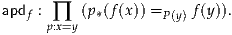


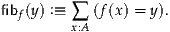
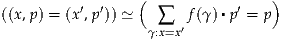
 .
.


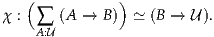

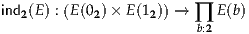


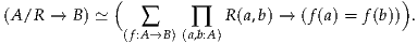


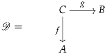
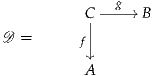

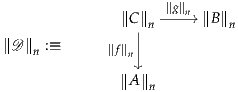
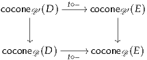


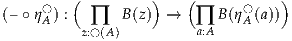


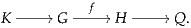
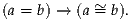

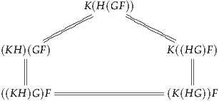
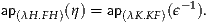
 hom
hom 


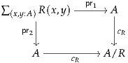

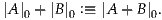
 " >
" >