http://people.csail.mit.edu/jaffer/Cell/CAN4S3
	4-Neighbor 3-State Universal Cellular Automaton

Described here is a infinitely-configurable universal (Turing machine) automaton. Its equilateral triangular cells tile the plane and are isotropic; the transitions for each cell depends only on (itself and) the multiplicities of the values in the three cells directly abutting it. Generations are discrete; all cells switch to their successor states simultaneously.

Table 1 - State Transition Rules

rule	neighbors	cell	->	next	(used for)
[j]	444	0	->	4	(junction repair)
[d]	441	4	->	1	(junction)
[k]	441	0	->	4	(junction)
[e]	440	1	->	0	(junction)
[g]	440	0	->	4	(gap repair, collision, and junction)
[f]	411	0	->	4	(junction)
[c]	410	0	->	4	(wire)
[a]	410	4	->	1	(wire)
[i]	410	1	->	0	(junction)
[b]	400	1	->	0	(wire)
[h]	100	1	->	4	(collision, junction)
[m]	100	4	->	1	(repair wire end; period 3 oscillator)
[n]	000	1	->	4	(repair wire end)
rest	???	x	->	x	(no change)

There are 10 possible combinations of states of three neighbors. Times the 3 possible states of the cell itself yields 30 possible transitions. Only the transitions which change the cell's state are listed; the others leave it unchanged.

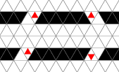
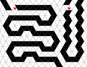
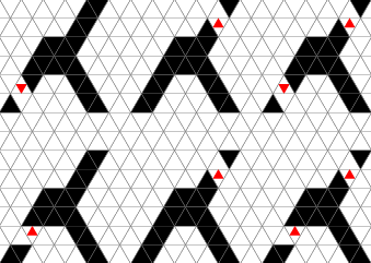
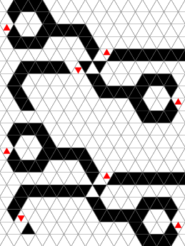
In the automata diagrams state "1" is coded by red (half-size triangle), state "4" by black, and state "0" by white. In figure 1 nine successive generations scanning from the top left to right are shown. Subsequent figures show just the initial state and are linked to PDFs showing one generation per page.

There are interesting symmetries in the application of these rules to the examples here.

• "4" never becomes "0";
• "1" never stays "1"; and
• "0" never becomes "1".

Figure 1 - Signal Propagation

Rules [a], [b], and [c] are needed for signal propagation in wires shown in figure 1. Wires can bend 60 degrees. A bend behaves like a straight wire because the rules do not distinguish between one neighbor and another. The minimum radius is 2; a turn can wrap around the minimal hexagon.

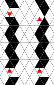
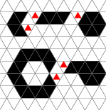
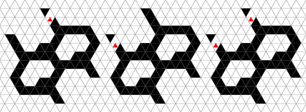
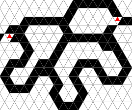
Figure 2

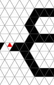
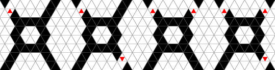
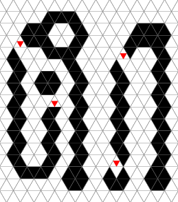
Figure 3

Two signals which meet on a wire annihilate each other. Both possible phases of such meetings are shown in figure 2. Notice that the center triangle of the upper wire never changes from black. This behavior of rule [e] will be important later. Figure 3 shows annihilations in wiggly wires.

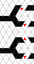
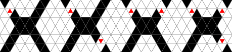
Figure 4

Three wires along different axes meeting at a single cell constitute a junction. Due to the gap repair rule [i] and the small neighborhood, wires must come into junctions at 120 degree angles from each other. Additional bends can be spaced 2 cells or further from the junction. Figure 4 shows two junctions the minimum distance apart.

Rules [d], [e], [f], and [g] give the junction the property that a signal coming in on one leg exits via the other two; demonstrated twice in figure 4. The minimum distance between junction points such that they don't interfere is 3.

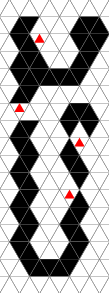
Figure 5

Two signals arriving simultaneously at a junction annihilate each other as shown in the top of figure 5.

Rule [i] allows the junction to function even if the signals are one step out of phase on arrival. The result, as shown in the bottom of figure 6 is that one signal exits on the remaining leg. This is in effect the same as if the delayed signal were delayed more than one step; being annihilated by the earlier signal having split through the junction.

Logic Elements

Figure 6 - Delay elements

Time delays are formed from serpentine wires as shown in figure 6.

Figure 7

An oscillator is formed of a wire loop and a junction. A pulse circulates in the loop and splits every time it passes through the junction. Figure 7 shows a period 6 clock and a period 18 clock.

Figure 8 - Hybrid Combiner

Figure 8 shows a four legged hybrid combiner. It is named for the radio-frequency component which couples adjacent ports while isolating opposite ports. It has the properties:

• A pulse on just one leg exits on the two adjacent legs;
• pulses on opposite legs exit on their two adjacent legs;
• pulses on adjacent legs exit on the two opposite legs; and
• three simultaneous pulses combine to one exiting the other leg.

Figure 9 - hybrid combiner

Like the oscillators in figure 7, hybrid combiners can be reduced to the minimum hexagonal form shown in figure 9.

Figure 10 - OR and Exclusive-OR Gates

The hybrid combiner can function as an OR gate as shown in the top half of figure 10. With a one cycle offset between (possible) input pulses, the hybrid combiner acts as an exclusive-or gate; shown in the bottom half of figure 10.

Figure 11 - Crossover

Three exclusive-or gates can be combined to form a crossover routing each of two inputs to its opposite wire; shown in figure 11.

Figure 12 - Switched Clock

An oscillator with a hybrid combiner forms a startable and stoppable clock. Period 18 and period 6 clocks are shown in figure 12.

Figure 13

Combining the hybrid with an oscillator in a different way creates an inverter (a "not" gate) as shown in figure 13. The first, six, and seventh pulses from the oscillator are annihilated.

Alignment

Figure 14 - Synchronizer

The synchronizer is an inverter allowing variation of input timing with respect to its period. Two 18-cycle oscillators feed a hybrid combiner so that their pulses cancel on the input side and produce a pulse on the output. An input pulse splits onto the clock legs, but does not emerge from the output side. Those pulses meet and annihilate clock pulses, and thus prevent the output pulse-to-be.

The two synchronizers in figure 14 receive pulses at different times showing the full 12-clock (out of 18) window for inputs to suppress the synchronized output pulse. Notice that the sequence of pulses exiting to right is the same, even though the input pulse arrivals differ by 12 generations.

Universality

Figure 15 - CCITT 16-bit CRC

Praxis

The machinery of mathematical proofs rarely makes practical devices. What sort of computations is this automaton suited for?

• Acting as storage, long folded delays lines (wires) approach 1/6 bit per cell in density. Individual bit storage would require 15 cells at a minimum; a hexagon plus half of its shared 18-cell border.

• With a crossover 15 times larger than an exclusive-or gate, bit-parallel busses would be space-inefficient. But serial logic is small and quite well suited to delay-line storage.