Tracking targets as a max-flow problem

Figure 11: a) A 2D office like environment. A single robot follows the green path. Red dots are illustrations of possible targets in the environment. b) The shadow sequence I-state for the environment and path. The orange indexed shadows are these at $t = t_0$ or appearing; the green ones are these at $t = t_f$ or disappearing. Shadow $s_{18}$ are both appearing and existing at $t = t_f$ . c) The bipartite I-state. d) Augmented graph for running max-flow algorithm.

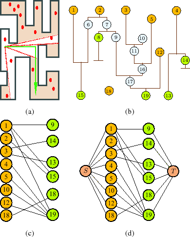
We now provide a concrete example to illustrate the combinatorial filtering process and the last step of the algorithm of applying a maximum flow algorithm (such as Edmonds-Karp). For the environment given in Fig. 11(a), visibility cell decomposition procedure [5] will give us the shadow sequence I-state in Fig. 11(b). Applying the $\mathcal I_{bip}$ filter then gives us the bipartite graph in Fig. 11(c). Note that each shadow becomes a vertex (sometimes two vertices) of the bipartite graph. Once the bipartite graph is constructed, the task of determining lower and upper bounds on shadows at $t = t_f$ can be transformed into a max-flow problem. To achieve this, we first augment the graph by adding a source vertex $S$ and sink vertex $T$ . An edge is added between $S$ and each shadow at $t = t_0$ as well as each appeared shadow, and an edge is added between $T$ and each shadow at $t = t_f$ as well as each disappeared shadow. The end result of doing this to the graph in Fig. 11(c) is Fig. 11(d).

After obtaining the extended graph, capacities need to be assigned to edges of the graph before running max-flow. Let $e(v_1, v_2)$ be an edge in the graph from vertex $v_1$ to vertex $v_2$ , and denote the capacity and flow on the edge as $c(v_1, v_2), f(v_1, v_2)$ , respectively. Suppose that we want to obtain the upper bound on the number of targets in shadow $s_{19}$ . The edges of the original bipartite graph will always have infinite capacities, which we do not mention again. For each edge between $S$ and and a shadow indexed $i$ , let $c(S, i) = u_i$ . In our example these indices are 1-5, 10, 12, and 18. For each edge between a disappearing shadow indexed $i$ , and $T$ , let $c(i, T) = u_i$ . These are 9 and 14 in our example. Since we want as many targets to go to $s_{19}$ as possible, we let $c(i, T) = 0$ for $i = 13, 15, 18$ and $c(19, T) = +\infty$ . After running the max-flow algorithm, the maximum possible number of targets that can end up in $s_{19}$ is given by

$$f(19, T) + \sum_if(i, T) - \sum_ic(i, T),$$ (7)

in which the summations are over indices of disappearing shadows. We need to consider disappearing shadows since these shadows must have flow equal to their capacity. If we instead want the lower bound on the number of targets in $s_{19}$ , we should let $c(S, i) = l_i$ , $c(i, T) = l_i$ for $i = 9, 14$ , $c(i, T) = +\infty$ for $i = 13, 15, 18$ and $c(19, T) = 0$ . After running the max-flow algorithm, $s_{19}$ 's lower bound is given by

$$\sum_ic(S, i) - \sum_{i}f(i, T),$$ (8)

in which the summations are over all applicable shadows. The same procedure applies to a set of shadows.