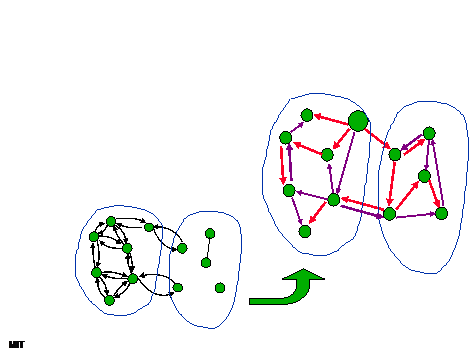
1	Randomization in Graph Optimization Problems David Karger MIT http://theory.lcs.mit.edu/~karger
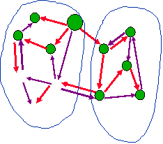
2	Randomized Algorithms Flip coins to decide what to do next Avoid hard work of making “right” choice Often faster and simpler than deterministic algorithms Different from average-case analysis Input is worst case Algorithm adds randomness
3	Methods Random selection if most candidate choices “good”, then a random choice is probably good Random sampling generate a small random subproblem solve, extrapolate to whole problem Monte Carlo simulation simulations estimate event likelihoods Randomized Rounding for approximation
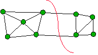
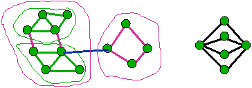
4	Cuts in Graphs Focus on undirected graphs A cut is a vertex partition Value is number (or total weight) of crossing edges
5	Optimization with Cuts Cut values determine solution of many graph optimization problems: min-cut / max-flow multicommodity flow (sort-of) bisection / separator network reliability network design Randomization helps solve these problems
6	Presentation Assumption For entire presentation, we consider unweighted graphs (all edges have weight/capacity one) All results apply unchanged to arbitrarily weighted graphs Integer weights = parallel edges Rational weights scale to integers Analysis unaffected Some implementation details
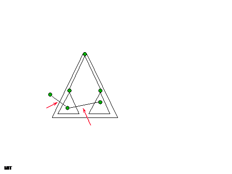
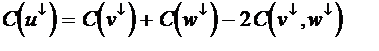
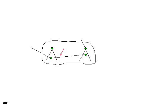
7	Basic Probability Conditional probability Pr[A Ç B] = Pr[A] × Pr[B \| A] Independent events multiply: Pr[A Ç B] = Pr[A] × Pr[B] Union Bound Pr[X È Y] £ Pr[X] + Pr[Y] Linearity of expectation: E[X + Y] = E[X] + E[Y]
8	Random Selection for Minimum Cuts Random choices are good when problems are rare
9	Minimum Cut Smallest cut of graph Cheapest way to separate into 2 parts Various applications: network reliability (small cuts are weakest) subtour elimination constraints for TSP separation oracle for network design Not s-t min-cut
10	Max-flow/Min-cut s-t flow: edge-disjoint packing of s-t paths s-t cut: a cut separating s and t [FF]: s-t max-flow = s-t min-cut max-flow saturates all s-t min-cuts most efficient way to find s-t min-cuts [GH]: min-cut is “all-pairs” s-t min-cut find using n flow computations
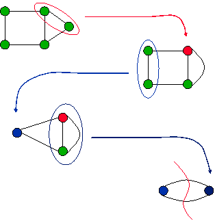
11	Flow Algorithms Push-relabel [GT]: push “excess” around graph till it’s gone max-flow in O^(mn) (note: O^ hides logs) recent O^(m^3/2) [GR] min-cut in O^(mn²) --- “harder” than flow Pipelining [HO]: save push/relabel data between flows min-cut in O^*(mn) --- “as easy” as flow
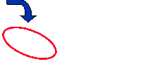
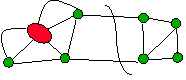
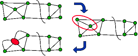
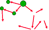
12	Contraction Find edge that doesn’t cross min-cut Contract (merge) endpoints to 1 vertex
13	Contraction Algorithm Repeat n - 2 times: find non-min-cut edge contract it (keep parallel edges) Each contraction decrements #vertices At end, 2 vertices left unique cut corresponds to min-cut of starting graph
14
15	Picking an Edge Must contract non-min-cut edges [NI]: O(m) time algorithm to pick edge n contractions: O(mn) time for min-cut slightly faster than flows If only could find edge faster….
16	Randomize Repeat until 2 vertices remain pick a random edge contract it (keep fingers crossed)
17	Analysis I Min-cut is small---few edges Suppose graph has min-cut c Then minimum degree at least c Thus at least nc/2 edges Random edge is probably safe Pr[min-cut edge] £ c/(nc/2) = 2/n (easy generalization to capacitated case)
18	Analysis II Algorithm succeeds if never accidentally contracts min-cut edge Contracts #vertices from n down to 2 When k vertices, chance of error is 2/k thus, chance of being right is 1-2/k Pr[always right] is product of probabilities of being right each time
19	Analysis III
20	Repetition Repetition amplifies success probability basic failure probability 1 - 2/n² so repeat 7n² times
21	How fast? Easy to perform 1 trial in O(m) time just use array of edges, no data structures But need n² trials: O(mn²) time Simpler than flows, but slower
22	An improvement [KS] When k vertices, error probability 2/k big when k small Idea: once k small, change algorithm algorithm needs to be safer but can afford to be slower Amplify by repetition! Repeat base algorithm many times
23	Recursive Algorithm Algorithm RCA ( G, n ) {G has n vertices} repeat twice randomly contract G to n/2^½ vertices RCA(G,n/2^1/2)
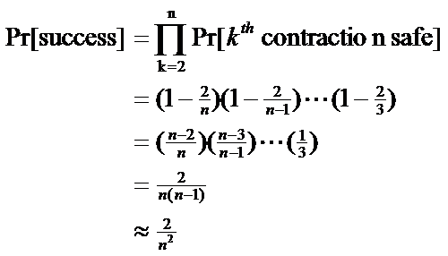
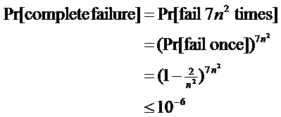
24	Main Theorem On any capacitated, undirected graph, Algorithm RCA runs in O^*(n²) time with simple structures finds min-cut with probability ³ 1/log n Thus, O(log n) repetitions suffice to find the minimum cut (failure probability 10^-6) in O(n²log² n) time.
25	Proof Outline Graph has O(n²) (capacitated) edges So O(n²) work to contract, then two subproblems of size n/2^½ T(n) = 2 T(n/2^½) + O(n²) = O(n² log n) Algorithm fails if both iterations fail Iteration succeeds if contractions and recursion succeed P(n)=1 - [1 - ½ P(n/2^½)]²= W (1 / log n)
26	Failure Modes Monte Carlo algorithms always run fast and probably give you the right answer Las Vegas algorithms probably run fast and always give you the right answer To make a Monte Carlo algorithm Las Vegas, need a way to check answer repeat till answer is right No fast min-cut check known (flow slow!)
27	How do we verify a minimum cut?
28	Enumerating Cuts The probabilistic method, backwards
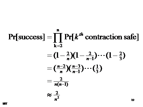
29	Cut Counting Original CA finds any given min-cut with probability at least 2/n(n-1) Only one cut found Disjoint events, so probabilities add So at most n(n-1)/2 min-cuts probabilities would sum to more than one Tight Cycle has exactly this many min-cuts
30	Enumeration RCA as stated has constant probability of finding any given min-cut If run O(log n) times, probability of missing a min-cut drops to 1/n³ But only n² min-cuts So, probability miss any at most 1/n So, with probability 1-1/n, find all O(n² log³ n) time
31	Generalization If G has min-cut c, cut £ac is a-mincut Lemma: contraction algorithm finds any given a-mincut with probability W (n^-2^a) Proof: just add a factor to basic analysis Corollary: O(n²^a) a-mincuts Corollary: Can find all in O^*(n²^a) time Just change contraction factor in RCA
32	Summary A simple fast min-cut algorithm Random selection avoids rare problems Generalization to near-minimum cuts Bound on number of small cuts Probabilistic method, backwards
33	Random Sampling
34	Random Sampling General tool for faster algorithms: pick a small, representative sample analyze it quickly (small) extrapolate to original (representative) Speed-accuracy tradeoff smaller sample means less time but also less accuracy
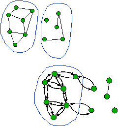
35	A Polling Problem Population of size m Subset of c red members Goal: estimate c Naïve method: check whole population Faster method: sampling Choose random subset of population Use relative frequency in sample as estimate for frequency in population
36	Analysis: Chernoff Bound Random variables X_iÎ [0,1] Sum X = å X_i Bound deviation from expectation Pr[ \|X-E[X]\| ³ e E[X] ] < exp(-e²E[X] / 4) “Probably, X Î (1±e) E[X]” If E[X] ³ 4(ln n)/e², “tight concentration” Deviation by e probability < 1 / n
37	Application to Polling Choose each member with probability p Let X be total number of reds seen Then E[X]=pc So estimate ĉ by X/p Note ĉ accurate to within 1±e iff X is within 1±e of expectation: ĉ = X/p Î (1±e) E[X]/p = (1±e) c
38	Analysis Let X_i=1 if i^th red item chosen, else 0 Then X= å X_i Chernoff Bound applies Pr[deviation by e] < exp(-e²pc/ 4) < 1/n if pc > 4(log n)/e² Pretty tight if pc < 1, likely no red samples so no meaningful estimate
39	Sampling for Min-Cuts
40	Min-cut Duality [Edmonds]: min-cut=max tree packing convert to directed graph “source” vertex s (doesn’t matter which) spanning trees directed away from s [Gabow] “augmenting trees” add a tree in O^(m) time min-cut c (via max packing) in O^(mc) great if m and c are small…
41	Example
42	Random Sampling Gabow’s algorithm great if m, c small Random sampling reduces m, c scales cut values (in expectation) if pick half the edges, get half of each cut So find tree packings, cuts in samples
43	Sampling Theorem Given graph G, build a sample G(p) by including each edge with probability p Cut of value v in G has expected value pv in G(p) Definition: “constant” r= 8 (ln n) / e² Theorem: With high probability, all exponentially many cuts in G(r/ c) have (1 ± e) times their expected values.
44	A Simple Application [Gabow] packs trees in O^(mc) time Build G(r/ c) minimum expected cut r by theorem, min-cut probably near r find min-cut in O^(r m) time using [Gabow] corresponds to near-min-cut in G Result: (1+e) times min-cut in O^*(m/e²) time
45	Proof of Sampling: Idea Chernoff bound says probability of large deviation in cut value is small Problem: exponentially many cuts. Perhaps some deviate a great deal Solution: showed few small cuts only small cuts likely to deviate much but few, so Chernoff bound applies
46	Proof of Sampling Sampled with probability r /c, a cut of value ac has mean ar [Chernoff]: deviates from expected size by more than e with probability at most n^-³^a At most n²^acuts have value ac Pr[any cut of value ac deviates] = O(n^-a) Sum over all a ³ 1
47	Las Vegas Algorithms Finding Good Certificates
48	Approximate Tree Packing Break edges into c /r random groups Each looks like a sample at rate r/ c O^( rm / c) edges each has min expected cut r so theorem says min-cut (1 – e) r So each has a packing of size (1 – e) r [Gabow] finds in time O^(r²m/c) per group so overall time is (c /r ) × O^(r²m/c) = O^(rm)
49	Las Vegas Algorithm Packing algorithm is Monte Carlo Previously found approximate cut (faster) If close, each “certifies” other Cut exceeds optimum cut Packing below optimum cut If not, re-run both Result: Las Vegas, expected time O^*(rm)
50	Exact Algorithm Randomly partition edges in two groups each like a ½ -sample: e = O^(c^-^½) Recursively pack trees in each half c/2 - O^(c^½) trees Merge packings gives packing of size c - O^(c^½) augment to maximum packing: O^(mc^½) T(m,c)=2T(m/2,c/2)+O^(mc^½) = O^(mc^½)
51	Nearly Linear Time
52	Analyze Trees Recall: [G] packs c (directed)-edge disjoint spanning trees Corollary: in such a packing, some tree crosses min-cut only twice To find min-cut: find tree packing find smallest cut with 2 tree edges crossing
53	Constraint trees Min-cut c: c directed trees 2c directed min-cut edges On average, two min-cut edges/tree Definitions: tree 2-crosses cut
54	Finding the Cut From crossing tree edges, deduce cut Remove tree edges
55	Two Problems Packing trees takes too long Gabow runtime is O^*(mc) Too many trees to check Only claimed that one (of c) is good Solution: sampling
56	Sampling Use G(r/c) with e=1/8 pack O^(r) trees in O^(m) time original min-cut has (1+e)r edges in G(r/ c) some tree 2-crosses it in G(r / c) …and thus 2-crosses it in G Analyze O^(r) trees in G time O^(m) per tree Monte Carlo
57	Simple First Step Discuss case where one tree edge crosses min-cut
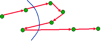
58	Analyzing a tree Root tree, so cut subtree Use dynamic program up from leaves to determine subtree cuts efficiently Given cuts at children of a node, compute cut at parent Definitions: v^¯ are nodes below v C(v^¯) is value of cut at subtree v^¯
59	The Dynamic Program
60	Algorithm: 1-Crossing Trees Compute edges’ LCA’s: O(m) Compute “cuts” at leaves Cut values = degrees each edge incident on at most two leaves total time O(m) Dynamic program upwards: O(n) Total: O(m+n)
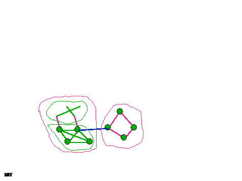
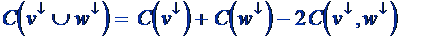
61	2-Crossing Trees Cut corresponds to two subtrees:
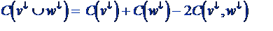
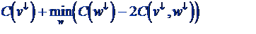
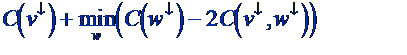
62	Linear Time Bottleneck is C(v^¯, w^¯) computations Avoid. Find right “twin” w for each v
63	How do we verify a minimum cut?
64	Network Design Randomized Rounding
65	Problem Statement Given vertices, and cost c_vw to buy and edge from v to w, find minimum cost purchase that creates a graph with desired connectivity properties Example: minimum cost k-connected graph. Generally NP-hard Recent approximation algorithms [GW],[JV]
66	Integer Linear Program Variable x_vw=1 if buy edge vw Solution cost S x_vwc_vw Constraint: for every cut, S x_vw³ k Relaxing integrality gives tractable LP Exponentially many cuts But separation oracles exist (eg min-cut) What is integrality gap?
67	Randomized Rounding Given LP solution values x_vw Build graph where vw is present with probability x_vw Expected cost is at most opt: S x_vwc_vw Expected number of edges crossing any cut satisfies constraint If expected number large for every cut, sampling theorem applies
68	k-connected subgraph Fractional solution is k-connected So every cut has (expected) k edges crossing in rounded solution Sampling theorem says every cut has at least k-(k log n)^1/2 edges Close approximation for large k Can often repair: e.g., get k-connected subgraph at cost 1+((log n)/k)^1/2 times min
69	Repair Methods Slightly increase all x_vw before rounding E.g., multiply by (1+e) Works fine, but some x_vw become > 1 Problem if only want single use of edges Round to approx, then fix Solve “augmentation problem” using other network design techniques May be worse approx, but only to a small part of cost
70	Nonuniform Sampling Concentrate on the important things [Benczur-Karger, Karger, Karger-Levine]
71	s-t Min-Cuts Recall: if G has min-cut c, then in G(r/c) all cuts approximate their expected values to within e. Applications:
72	The Problem Cut sampling relied on Chernoff bound Chernoff bounds required that no one edge is a large fraction of the expectation of a cut it crosses If sample rate <<1/c, each edge across a min-cut is too significant
73	Biased Sampling Original sampling theorem weak when large m small c But if m is large then G has dense regions where c must be large where we can sample more sparsely
74	Problem Old Time New Time Approx. s-t min-cut O^(mv) O^(nv/e²) Approx. s-t min-cut O^(mn) O^(n²/e²) Approx. s-t max-flow O^(m^3/2) O^(mn^1/2/e) Flow of value v O^(mv) O^(nv) m Þ n/e² in weighted, undirected graphs
75	Strong Components Definition: A k-strong component is a maximal vertex-induced subgraph with min-cut k.
76	Nonuniform Sampling Definition: An edge is k-strong if its endpoints are in same k-component. Stricter than k-connected endpoints. Definition: The strong connectivity c_e for edge e is the largest k for which e is k-strong. Plan: sample dense regions lightly
77	Nonuniform Sampling Idea: if an edge is k-strong, then it is in a k-connected graph So “safe” to sample with probability 1/k Problem: if sample edges with different probabilities, E[cut value] gets messy Solution: if sample e with probability p_e, give it weight 1/p_e Then E[cut value]=original cut value
78	Compression Theorem Definition: Given compression probabilities p_e, compressed graph G[p_e] includes edge e with probability p_e and gives it weight 1/p_eif included Note E[G[p_e]] = G Theorem: G[r / c_e] approximates all cuts by e has O(rn) edges
79	Application Compress graph to rn=O^(n/e²) edges Find s-t max-flow in compressed graph Gives s-t mincut in compressed So approx. s-t mincut in original Assorted runtimes: [GT] O(mn) becomes O^(n²/e²) [FF] O(mv) becomes O(nv/e²) [GR] O(m^3/2) become O(n³^/²/e³)
80	Proof (approximation) Basic idea: in a k-strong component, edges get sampled with prob. r / k original sampling theorem works Problem: some edges may be in stronger components, sampled less Induct up from strongest components: apply original sampling theorem inside then “freeze” so don’t affect weaker parts
81	Strength Lemma Lemma: å 1/c_e £ n Consider connected component C of G Suppose C has min-cut k Then every edge e in C has c_e ³ k So k edges crossing C’s min-cut have å 1/c_e £ å 1/k £ k (1/k ) = 1 Delete these edges (“cost” 1) Repeat n - 1 times: no more edges!
82	Proof (edge count) Edge eincluded with probability r / c_e So expected number is S r / c_e We saw S 1/c_e £ n So expected number at most r n
83	Construction To sample, must find edge strengths can’t, but approximation suffices Sparse certificates identify weak edges: construct in linear time [NI] contain all edges crossing cuts £ k iterate until strong components emerge Iterate for 2ⁱ-strong edges, all i tricks turn it strongly polynomial
84	NI Certificate Algorithm Repeat k times Find a spanning forest Delete it Each iteration deletes one edge from every cut (forest is spanning) So at end, any edge crossing a cut of size £ k is deleted [NI] pipeline all iterations in O(m) time
85	Approximate Flows Uniform sampling led to tree algorithms Randomly partition edges Merge trees from each partition element Compression problematic for flow Edge capacities changed So flow path capacities distorted Flow in compressed graph doesn’t fit in original graph
86	Smoothing If edge has strength c_e, divide into br / c_e edges of capacity c_e /br Creates br å 1/c_e= brn edges Now each edge is only 1/br fraction of any cut of its strong component So sampling a 1/b fraction works So dividing into b groups works Yields (1-e) max-flow in O^*(mn^1/2/e) time
87	Exact Flow Algorithms Sampling from residual graphs
88	Residual Graphs Sampling can be used to approximate cuts and flows A non-maximum flow can be made maximum by augmenting paths But residual graph is directed. Can sampling help? Yes, to a limited extent
89	First Try Suppose current flow value f residual flow value v-f Lemma: if all edges sampled with probability rv/c(v-f) then, w.h.p., all directed cuts within e of expectations Original undirected sampling used r/c Expectations nonzero, so no empty cut So, some augmenting path exists
90	Application When residual flow i, seek augmenting path in a sample of mrv/ic edges. Time O(mrv/ic). Sum over all i from v down to 1 Total O(mrv (log v)/c) since S1/i=O(log v) Here, e can be any constant < 1 (say ½) So r=O(log n) Overall runtime O^*(mv/c)
91	Proof Augmenting a unit of flow from s to t decrements residual capacity of each s-t cut by exactly one
92	Analysis Each s-t cut loses f edges, had at least v So, has at least ( v-f ) / v times as many edges as before But we increase sampling probability by a factor of v / ( v-f ) So expected number of sampled edges no worse than before So Chernoff and union bound as before
93	Strong Connectivity Drawback of previous: dependence on minimum cut c Solution: use strong connectivities Initialize a=1 Repeat until done Sample edges with probabilities ar / k_e Look for augmenting path If don’t find, double a
94	Analysis Theorem: if sample with probabilities ar/k_e, and a > v/(v-f), then will find augmenting path w.h.p. Runtime: a always within a factor of 2 of “right” v/(v-f) As in compression, edge count O(a r n) So runtime O(r n S_iv/i)=O^*(nv)
95	Summary Nonuniform sampling for cuts and flows Approximate cuts in O(n²) time for arbitrary flow value Max flow in O(nv) time only useful for “small” flow value but does work for weighted graphs large flow open
96	Network Reliability Monte Carlo estimation
97	The Problem Input: Graph G with n vertices Edge failure probabilities For exposition, fix a single p Output: FAIL(p): probability G is disconnected by edge failures
98	Approximation Algorithms Computing FAIL(p) is #P complete [V] Exact algorithm seems unlikely Approximation scheme Given G, p, e, outputs e-approximation May be randomized: succeed with high probability Fully polynomial (FPRAS) if runtime is polynomial in n, 1/e
99	Monte Carlo Simulation Flip a coin for each edge, test graph k failures in t trials Þ FAIL(p) » k/t E[k/t] = FAIL(p) How many trials needed for confidence? “bad luck” on trials can yield bad estimate clearly need at least 1/FAIL(p) Chernoff bound: O^(1/e²FAIL(p)) suffice to give probable accuracy within e Time O^(m/e²FAIL(p))
100	Chernoff Bound Random variables X_iÎ [0,1] Sum X = å X_i Bound deviation from expectation Pr[ \|X-E[X]\| ³ e E[X] ] < exp(-e²E[X] / 4) If E[X] ³ 4(log n)/e², “tight concentration” Deviation by e probability < 1 / n No one variable is a big part of E[X]
101	Application Let X_i=1 if trial i is a failure, else 0 Let X = X₁ + … + X_t Then E[X] = t · FAIL(p) Chernoff says X within relative e of E[X] with probability 1-exp(e²t FAIL(p)/4) So choose t to cancel other terms “High probability” t = O(log n / e²FAIL(p)) Deviation by e with probability < 1 / n
102	For network reliability Random edge failures Estimate FAIL(p) = Pr[graph disconnects] Naïve Monte Carlo simulation Chernoff bound---“tight concentration” Pr[ \|X-E[X]\| £ e E[X] ] < exp(-e²E[X] / 4) O(log n / e²FAIL(p)) trials expect O(log n / e²) network failures---sufficient for Chernoff So estimate within e in O^*(m/e²FAIL(p)) time
103	Rare Events When FAIL(p) too small, takes too long to collect sufficient statistics Solution: skew trials to make interesting event more likely But in a way that let’s you recover original probability
104	DNF Counting Given DNF formula (OR of ANDs) (e₁ Ùe₂ Ù e₃) Ú (e₁ Ù e₄) Ú (e₂ Ù e₆) Each variable set true with probability p Estimate Pr[formula true] #P-complete [KL, KLM] FPRAS Skew to make true outcomes “common” Time linear in formula size
105	Rewrite problem Assume p=1/2 Count satisfying assignments “Satisfaction matrix Truth table with one column per clause S_ij=1 if i^th assignment satisfies j^th clause We want number of nonzero rows
106	Satisfaction Matrix
107	New sample space Normalize each nonzero row to one So sum of nonzeros is desired value Goal: estimate average nonzero Method: sample random nonzeros
108	Sampling Nonzeros We know number of nonzeros/column If satisfy given clause, all variables in clause must be true All other variables unconstrained Estimate average by random sampling Know number of nonzeros/column So can pick random column Then pick random true-for-column assignment
109	Few Samples Needed Suppose k clauses Then E[sample] > 1/k 1 £ satisfied clauses £ k 1 ³ sample value ³ 1/k Adding O(k log n / e²) samples gives “large” mean So Chernoff says sample mean is probably good estimate
110	Reliability Connection Reliability as DNF counting: Variable per edge, true if edge fails Cut fails if all edges do (AND of edge vars) Graph fails if some cut does (OR of cuts) FAIL(p)=Pr[formula true]
111	Focus on Small Cuts Fact: FAIL(p) > p^c Theorem: if p^c=1/n⁽²⁺^d⁾ then Pr[>a-mincut fails]< n^-^ad Corollary: FAIL(p) » Pr[£ a-mincut fails], where a=1+2/d Recall: O(n²^a) a-mincuts Enumerate with RCA, run DNF counting
112	Review Contraction Algorithm O(n²^a) a-mincuts Enumerate in O^*(n²^a) time
113	Proof of Theorem Given p^c=1/n⁽²⁺^d⁾ At most n²^acuts have value ac Each fails with probability p^a^c=1/n^a⁽²⁺^d⁾ Pr[any cut of value ac fails] = O(n^-a^d) Sum over all a > 1
114	Algorithm RCA can enumerate all a-minimum cuts with high probability in O(n²^a) time. Given a-minimum cuts, can e-estimate probability one fails via Monte Carlo simulation for DNF-counting (formula size O(n²^a)) Corollary: when FAIL(p)< n^-⁽²⁺^d⁾, can e-approximate it in O (cn^2+4/^d) time
115	Combine For large FAIL(p), naïve Monte Carlo For small FAIL(p), RCA/DNF counting Balance: e-approx. in O(mn^3.5/e²) time Implementations show practical for hundreds of nodes Again, no way to verify correct
116	Summary Naïve Monte Carlo simulation works well for common events Need to adapt for rare events Cut structure and DNF counting lets us do this for network reliability
117	Conclusions
118	Conclusion Randomization is a crucial tool for algorithm design Often yields algorithms that are faster or simpler than traditional counterparts In particular, gives significant improvements for core problems in graph algorithms
119	Randomized Methods Random selection if most candidate choices “good”, then a random choice is probably good Monte Carlo simulation simulations estimate event likelihoods Random sampling generate a small random subproblem solve, extrapolate to whole problem Randomized Rounding for approximation
120	Random Selection When most choices good, do one at random Recursive contraction algorithm for minimum cuts Extremely simple (also to implement) Fast in theory and in practice [CGKLS]
121	Monte Carlo To estimate event likelihood, run trials Slow for very rare events Bias samples to reveal rare event FPRAS for network reliability
122	Random Sampling Generate representative subproblem Use it to estimate solution to whole Gives approximate solution May be quickly repaired to exact solution Bias sample toward “important” or “sensitive” parts of problem New max-flow and min-cut algorithms
123	Randomized Rounding Convert fractional to integral solutions Get approximation algorithms for integer programs “Sampling” from a well designed sample space of feasible solutions Good approximations for network design.
124	Generalization Our techniques work because undirected graph are matroids All our results extend/are special cases Packing bases Finding minimum “quotients” Matroid optimization (MST)
125	Directed Graphs? Directed graphs are not matroids Directed graphs can have lots of minimum cuts Sampling doesn’t appear to work
126	Open problems Flow in O(n²) time Eliminate v dependence Apply to weighted graphs with large flows Flow in O(m) time? Las Vegas algorithms Finding good certificates Detrministic algorithms Deterministic construction of “samples” Deterministically compress a graph
127	Randomization in Graph Optimization Problems David Karger MIT http://theory.lcs.mit.edu/~karger karger@mit.edu