iSAM is my Ph.D. dissertation work that was advised by Frank Dellaert at the Georgia Institute of Technology. Back in 2005 I worked on data association and needed marginal covariances for the SLAM problem. Calculating those in the naive way yielded hour-long waiting times even for relatively small problems. At that time I got interested in ongoing work by Frank called Square Root SAM and finally helped with the experiments of the IJRR 2006 paper. Together with Ananth Ranganathan we figured out a way of recovering arbitrary parts of the full covariance matrix from the square root information factor that Square Root SAM calculates. However, calculating that square root information matrix itself from scratch eventually becomes expensive for larger problems. Instead, I started to incrementally update the square root information matrix, which is advantageous because most of the time new measurements only affect a small part of the variables of the SLAM problem. We eventually selected Givens rotations as a simple mechanism to update a QR matrix factorization, which gave rise to the iSAM algorithm, first published in IJCAI in January 2007.
In the iSAM library, we represent the SLAM problem as a factor graph. A factor graph is a bipartite graph that contains two types of nodes: variable nodes and factor nodes. Edges are only allowed between different types of nodes, i.e. they always connect a node with a factor. Here is an example of a factor graph representing a simple SLAM problem:

Colored circles represent variable nodes, and small solid black circles represent factor nodes. Robot poses x_i are marked blue and are connected by a chain of odometry measurements u_i. Other constraints, for example derived from laser scan-matching are not necessarily connecting subsequent poses, but can also encode loop closing constraints. So far the SLAM problem represents a so-called pose graph, consisting only of poses and constraints.
SLAM can also contain landmarks, here the landmark locations l_j shown in green. Landmark observations u_k are also represented by factors. Landmarks can for example be observed by laser range finders or cameras. The resulting optimization problem is referred to as bundle adjustment in photogrammetry and as structure from motion in computer vision.
While this example can readily be represented as a Bayes net, as typically found in the SLAM literature, more complicated scenarios are more easily represented as factor graphs. For example, the calibration of a sensor can be represented by another node that connects to all relevant factors. A more advanced example is provided by the concept of anchor nodes, see anchor nodes.
For a code example, please see the Simple iSAM Example.
The isam::Slam class in Slam.h represents the factor graph, providing methods for creating the graph as well as optimizing. Of particular interest are the methods isam::Slam::add_node() and isam::Slam::add_factor() that are needed to incrementally build the SLAM graph. Suitable nodes and factors for 2D SLAM problems can be found in slam2d.h. The method isam::Slam::update() performs the necessary calculations to obtain a new estimate, and is typically called after all factors of a time step are added. The detailed behavior of the algorithm can be controlled through isam::Slam::update_properties().
In many cases the iSAM library can automatically generate initial estimates for new nodes based on the first measurement that gets connected to the node. For odometry, for example, the current estimate of the previous pose together with the odometry measurement provides the initialization of the new pose. In other situations, such as when partial constraints are being added (eg. stereo measurements), multiple measurements might be needed to constrain the new variable (eg. camera pose). In that case the user can provide the initialization that was for example obtained by a RANSAC algorithm with 5-point algorithm. In that case the user can call isam::Node::init() with the appropriate estimate.
New types of factors can easily be defined by the user. Examples of factors are provided in slam2d.h. The user simply creates a new class derived from Factor and defines a cost function. To allow fast prototyping, iSAM by default uses numerical differentiation. For time-critical implementations, the user can optionally provide a symbolic derivative by overwriting isam::Factor::jacobian.
New types of nodes can also be defined by the user. Good examples of nodes are Point2d (simple) and Pose3d (more advanced). The user simply creates a new class that contains the variables to be optimized as well as an exponential map. In many cases the exponential map simply adds a delta vector to the variable. However, when dealing with overparametrized representations such as Quaternions, rotation matrices and homogeneous points (see Rot3d and Point3dh), the exponential map allows using a minimal representation within the optimization. The minimal representation is only needed locally for updates, while a global minimal representation might not be available or suitable for this purpose.
A key advantage of iSAM is the efficient access to the exact marginal covariances. See examples/covariances.cpp for how to access selected parts of the full marginal covariance matrix. Note that recovering the full marginal covariance is infeasible for large problems, independent of the algorithm used, as the matrix itself contains O(n^2) entries that would have to be calculated.
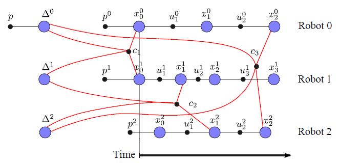
We have recently presented a novel approach to multi-robot or multi-session mapping. An implementation of anchor nodes is included in iSAM, for usage see examples/anchorNodes.cpp.

The figure shows three robot trajectories that are not synchronized, and do not require initial relative pose estimates. Encounters later define the alignment of the trajectories in a common frame. For more details please refer to: