Recovering position from distance measurements
— “Multilateration”
Each distance measurement confines possible positions for the
initiator (smartphone) to the surface of a sphere, defined by
$$
\|{\bf r}-{\bf r}_i\| = d_i
$$
where \({\bf r}=(x, y,z)\) is the position of the initiator,
\( {\bf r}_i = (x_i, y_i, z_i) \) the position of the \(i\)-th
responder (WiFi access point),
and \(d_i\) the distance between them.
This can obviously be written as a second order equation in the
components \(x, y,\) and \(z\):
$$
(x-x_i)^2 + (y-y_i)^2 + (z-z_i)^2 = d_i^2
$$
We can find the position of the smartphone by intersecting spheres.
Three spheres intersect in two points.
So with distances to three responders known there remains a two-way ambiguity,
which can be resolved if distance to a fourth responder is known.
This is analogous to finding cell towers from measurements of
LTE TimingAdvance on a smartphone:
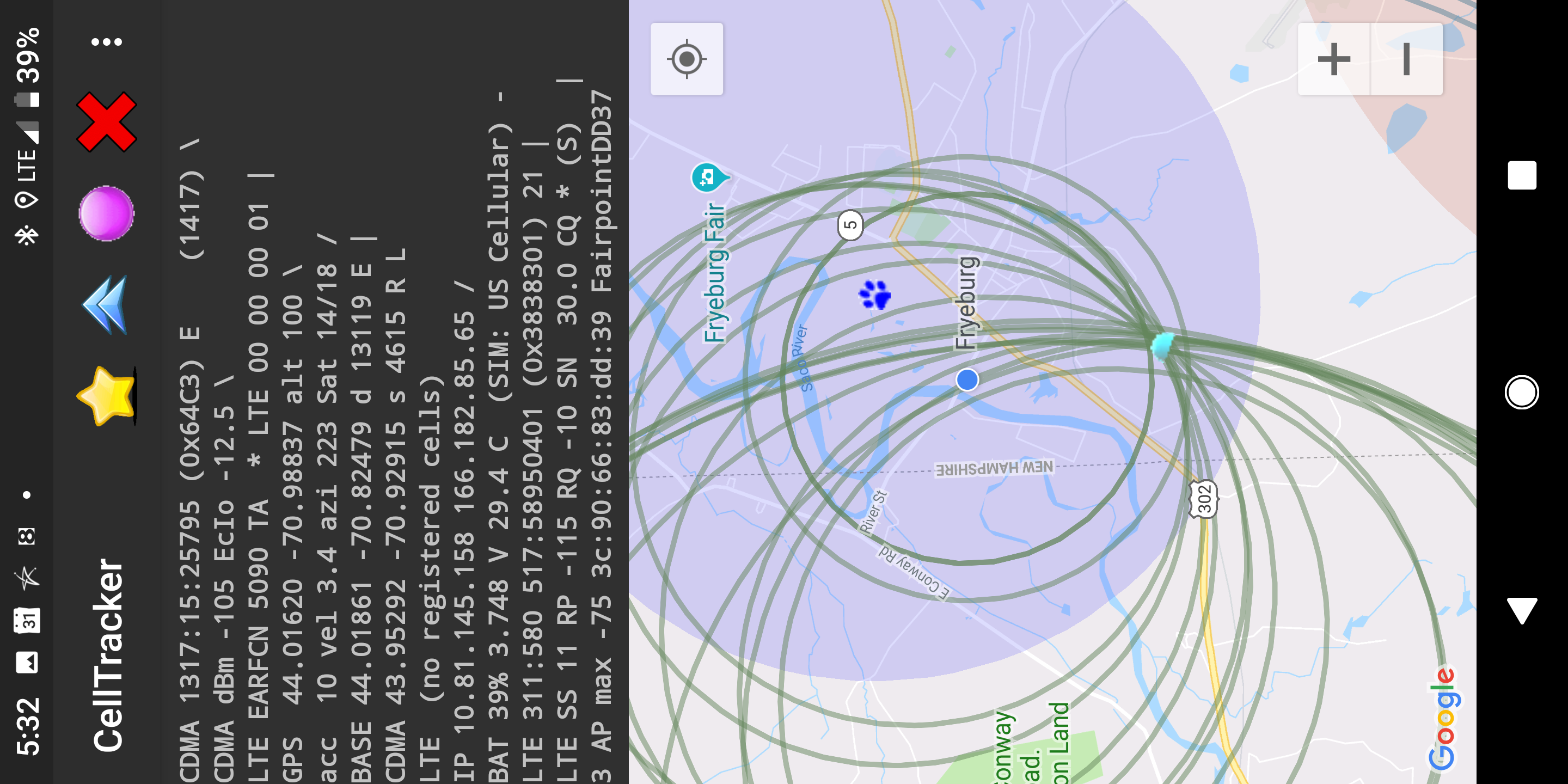 The circles in the screen shot above have centers at various cell phone
positions and radii corresponding to the LTE TimingAdvance reported
at those positions. The cyan spot is the actual position of the base station.
Two circles intersect in two points.
So with distances of the base station from two positions known, there remains
a two-way ambiguity,
which can be resolved if distances from three or more positions are known.
The circles in the screen shot above have centers at various cell phone
positions and radii corresponding to the LTE TimingAdvance reported
at those positions. The cyan spot is the actual position of the base station.
Two circles intersect in two points.
So with distances of the base station from two positions known, there remains
a two-way ambiguity,
which can be resolved if distances from three or more positions are known.
In the 3-D version of the problem,
each distance measurement provides one constraint, and so we expect a finite number of
solutions for the position when we have three measurements.
We can rewrite the above equation in the alternate form
$$
(x^2+y^2+z^2) - 2 (x_i x + y_i y + z_i z) = d_i^2 - (x_i^2+y_i^2+z_i^2)
$$
which makes it clear that we can obtain linear equations
in \(x, y,\) and \(z\)
by subtracting these equations pairwise.
However, the number of solutions with three responders is two,
since we can only reduce the three second order equations to two
linear equations with one remaining quadratic equation
(The three linear equation that could be obtained in this fashion are not linearly independent).
Actually, the two-way ambiguity will always occur when the responders lie in a common plane.
The reason is that the distances from responders to two points that are mirror images with respect
to a plane containing the responders are the same.
So in this case mirror images cannot be distinguished from sets of distance measurements alone.
It is, as a result, best not to have responders lying in a common plane
(or even worse, lined up in a straight line).
With four or more responders we have an overdetermined system and
— in the presence of measurement errors —
there is no longer a solution that satisfies all of the constraints.
We can then take one of several different approaches:
-
Implied linear equations and the pseudo inverse
(Spoiler alert: don't do this!)
Since linear equations are easy to deal with, it is tempting to extend the
above approach by subtracting second order equation
from one another to obtain linear equations in \(x, y,\) and \(z\):
$$
x (x_j - x_i) + y (y_j - y_i) + z (z_j - z_i) = \bigl((d_i^2 - d_j^2) - (R_i^2 -
R_j^2)\bigr)/2
$$
where
\( R_i^2 = x_i^2 + y_i^2 + z_i^2 \),
If there are \(N\) responders, we can do this for each of
\( M = N(N-1)/2 \) different pairs to obtain
$$
A {\bf r} = {\bf b},
$$
where \(A\) is a \(M\times3\) matrix.
With three responders we get three linearly dependent equations and so
cannot find a unique solution in this fashion
(even though we know that there are only two solutions to the
original problem for \(N=3\) in the 3-D case).
If \(N\) > 3, we obtain more equations than unknowns
(not all independent) and so are dealing with an overdetermined linear system.
In the special case of four responders, we can pick three independent rows
(out of the six),
obtain a \(3\times 3\) matrix \(A'\), and write \(A'{\bf r} = {\bf b}' \)
for
$$
\begin{pmatrix}
(x_1-x_0) & (y_1-y_0) & (z_1 - z_0)\\
(x_2-x_1) & (y_2-y_1) & (z_2 - z_1)\\
(x_3-x_2) & (y_3-y_2) & (z_3 - z_2)
\end{pmatrix}
\begin{pmatrix}x \\ y \\ z \end{pmatrix}
=
\frac{1}{2}
\begin{pmatrix}
(d_0^2-d_1^2) - (R_0^2-R_1^2) \\
(d_1^2-d_2^2) - (R_1^2-R_2^2) \\
(d_2^2-d_3^2) - (R_2^2-R_3^2) \\
\end{pmatrix}
$$
We can solve these three linear equations in three unknowns directly
using e.g. Gaussian elimination, of course.
More generally, this method can be used to set up a problem to minimize the
“error” \( \| A {\bf r} - {\bf b} \| \),
the solution of which is given by the
pseudo-inverse:
$$
{\bf r} = (A^TA)^{-1}A^T {\bf b}.
$$
This straightforward method does produce the correct position when given perfect
distance measurement data.
However, it has high “noise gain” when given real data.
That is, small errors in the input data produce large errors in the result.
(One way one can tell right away that this approach is “wrong”
is that the result is dependent on the choice of coordinate systems —
an offset in coordinates does not lead to an equal offset in the solution).
Conclusion: Don't do this!
An aside: this is quite analogous to the infamous
8-point method
in machine vision for solving the
Relative Orientation problem.
While it is very appealing because of the linear form of the equations,
minimization of errors in those equations does not minimize the
sum of errors in image positions
(See
What is Wrong with so-called 'Linear' Photogrammetric Methods?
and
Projective Geometry Considered Harmful).
As a result, this method can not be recommended (other than perhaps
in the hope of finding plausible starting values for methods that do
the right thing).
-
Least squares and gradient descent
We can use
least squares minimization directly
on the sum of squares of differences between measured distances and
actual distances computed for a given position.
$$
{{\rm min}\atop{\bf r}}
\sum_{i=1}^N
( \| {\bf r} - {\bf r}_i \| - d_i)^2
$$
There is no closed form solution to this minimization problem.
An extremum can be found iteratively by moving the position
\({\bf r}\) in
steps in a direction opposite to the gradient of the error.
The gradient is the vector
$$
\nabla(e) =
2\sum_{i=1}^N
( \| {\bf r} - {\bf r}_i \| - d_i)
{{\bf r} - {\bf r}_i \over \| {\bf r} - {\bf r}_i \|}
$$
where \(e\) is the sum of squares of errors above.
The iteration proceeds as
$$
{\bf r}^{(n+1)} = {\bf r}^{(n)} - \gamma \nabla(e)
$$
where \(\gamma\) controls the step size
(it is picked so that the total error is reduced).
Note that here the gradient is simply a weighted sum of unit vectors in the directions
to the responders, where the weights are the errors in distance.
Such simple gradient descent methods can be speeded up a lot
using
Newtons method
with the inverse of the Hessian matrix of partial derivatives of second order:
$$
{\bf r}^{(n+1)} = {\bf r}^{(n)} - H(e)^{-1} \nabla(e)
$$
where \(e\) is the sum of squares of errors,
where \(\nabla(e)\) the gradient of \(e\)
w.r.t. \(r\), and \(H(e)\) the Hessian matrix.
Unfortunately, the “error surface” can be quite contorted and
methods such as gradient descent can get stuck in local minima.
-
Brute force grid search
Typically, the ratio of search volume edge length (tens of meters
perhaps) to expected error (a meter or two) is not very
large, making an exhaustive search on a grid feasible.
While outdoors useable WiFi signals may be picked up from perhaps 50 or even
100 meters (particularly at the lower frequencies of the 2.4 GHz band),
in buildings, signals are attenuated so as to be hard to use after not much
more than perhaps 10 or 20 meter.
The expected accuracy in turn is only about a meter or two,
so a fairly coarse grid can be used.
An exhaustive search of the volume of interest on a grid with spacing
of say 0.25 meter need consider only a few hundred thousand
voxels.
This is something a smartphone can do much faster than the time it takes to
obtain the RTT measurement
(which is about 30 – 60 milliseconds per responder).
Given the error in the measurements, there is no guarantee that the global
minimum is the sought after answer, but in many cases it will be.
The quantized position resulting from the grid search could be used
as a starting point for either a finer grid search or a gradient descent search.
But, because of the magnitude of the error in the measurements, there
is no point in doing that.
-
Kalman Filtering
Kalman filtering
(Thiele 1880)
provides a way to update an estimate of the
position along with an estimate of the
covariance matrix of uncertainty in the estimated position
ever time a measurement is made.
It is based on assumptions of Gaussian noise independent of the
measurement,
Gaussian transition probabilities and linearity.
Unfortunately the
measurement error
is not Gaussian nor independent of the measurement itself.
Also, when near one of the responders, the area of likely positions is
shaped more like a kidney (i.e. part of a circular arc) than something that can be
well approximated by a linearly stretched out Gaussian distribution
(see Dilution of Precision).
-
Particle Filter
If the probability distribution is not easily modeled in some
parameterized way (such as a multi-dimensional Gaussian),
then other means may be used to represent it.
One such method is that of
particle filters
which uses weighted samples to represent a distribution.
The distribution is in effect approximated by the sum of weighted impulses.
At each step, the position of the particles is updated based on a transition model.
The weights of the particles are adjusted based on the measurements.
Particles with low weight are then discarded, while new particles
are sampled to keep the overall number of particles at a desired value.
-
Bayesian Grid Update
But, the method showing most promise is Bayesian Grid Update.
Click here to go back to
main article on FTM RTT.
Berthold K.P. Horn,
bkph@ai.mit.edu
Accessibility