
|
http://people.csail.mit.edu/jaffer/FreeSnell/polyethylene.html |
FreeSnell: Polyethylene | |
FreeSnell is a program to compute optical properties of multilayer thin-film coatings.
This validation suite is from "polyethylene.scm", part of the FreeSnell package. "polyethylene.log" is the text generated by running polyethylene.scm:
scm -l polyethylene.scm > polyethylene.log
In Radiative Cooling in Passive Cooling, edited by Jeffrey Cook (MIT Press, 1989, pp. 138-196. ISBN: 0262531712), M. Martin writes:
The only practical approach to an infrared-transparent glazing material at present appears to be thin sheets of polyolefin plastics, and high density polyethylene in particular.
In order to model a material, FreeSnell needs spectral refractive-indexes over the range of interest. Refractive indexes are typically ascertained using spectroscopic ellipsometry; but ellipsometry data for polyethylene does not seem to be available.
There are graphs of polyethylene's normal infrared transmission from many sources; but complex refractive-indexes can't be synthesized from a single scalar spectrum (lacking phase information). But data can be extracted from measurements of several thickness of films. Attenuation due to the complex part of the refractive index is proportional to the exponential of the thickness of the piece. The average attenuation due to the real part of the refractive index does not depend on material thickness.
And even if we had one set of spectral refractive-index data for polyethylene, it would be prudent to examine these graphs to see how much variation occurs depending on density, degree of crystallinity, and aging.
... the infrared transmissivity of polyethylene, which exhibits a continuum type of background emissivity in the spectral range of the atmospheric window.
An constant IR of 1.54+0.002i produces a curve with higher attenuation at shorter wavelengths. This is because the imaginary part (0.002i) of the refractive index is akin to conductance; at shorter wavelengths more cycles are "short circuited". But polyethylene is transparent at visible wavelengths; so its IR must vary with wavelength.
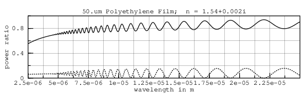
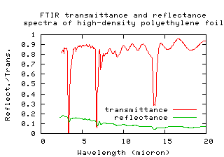
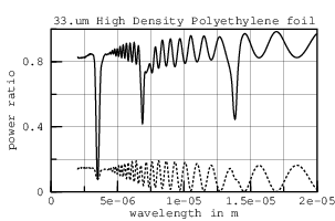
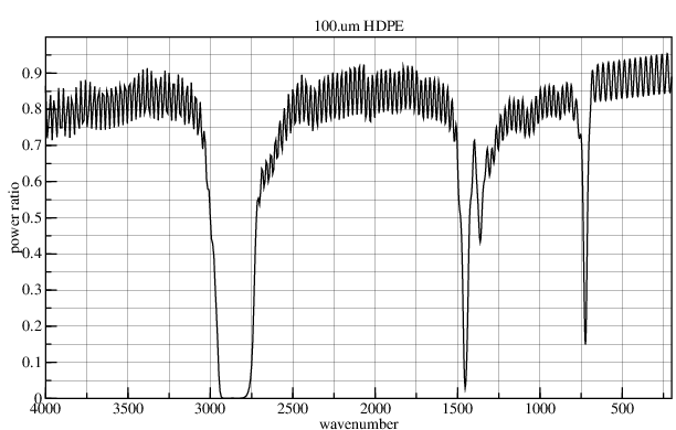
Figure 5 of TiO2 Nanocrystalline Pigmented Polyethylene Foils for Radiative Cooling Applications: Synthesis and Characterization by Y, Mastai et al (Langmuir,17, 22, 7118, 7123, 2001, 10.1021/la010370g), gives both reflectance and transmittance of a 100.um high-density polyethylene foil. The reflectance is the wedge which can separate the real and imaginary parts of the refractive index.
At 2.5.um, the reflectance plus the transmittance is 100 %. This leaves no room for loss; thus the extinction coefficient at 2.5.um must be 0. The reflectance rising with decreasing wavelength constrains the real part of the refractive index to rise over the interval 12.5.um to 2.5.um. Because the transmittance plus reflectance is less than 100 % at long wavelengths, there must be loss. This is modeled as the imaginary part rising from 0 to +0.002i over the range 2.5.um to 15.um.
 |
|
|---|---|
 | 
|
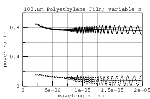
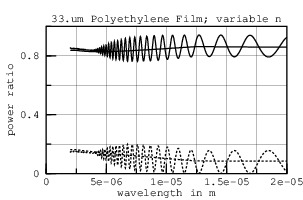
But the left graph disagrees with the published graph as to where the peaks and valleys of ripple are. Changing the thickness to 33.um brings them into close agreement. I can only conclude that their graph is mislabeled, and that their sample was actually 33.um thick.
While the reflection and transmission have opposing ripples in the constant IR graph at the top of this page, the transmission ripples of this graph are not opposed by equal reflection ripples. This could be due to the range of incidence angles for transmission and reflection measurements being different. In any case, the low resolution of this graph makes it a poor source for deriving detailed n and k values.
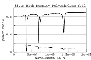
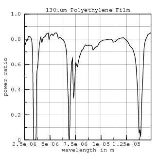
These experiments do make clear that the real part of HDPE's refractive index, n, varies slowly with wavelength. With n as a function of w now established, I can compute k from the transmission through a very thick (130.um) layer of HDPE in an approach suggested by Tsilingiris. The graphs including absorption lines with smoothed ripple and without ripple (using layer*) are:
|
|
|---|---|
 | 
|
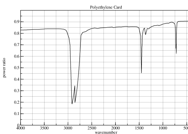
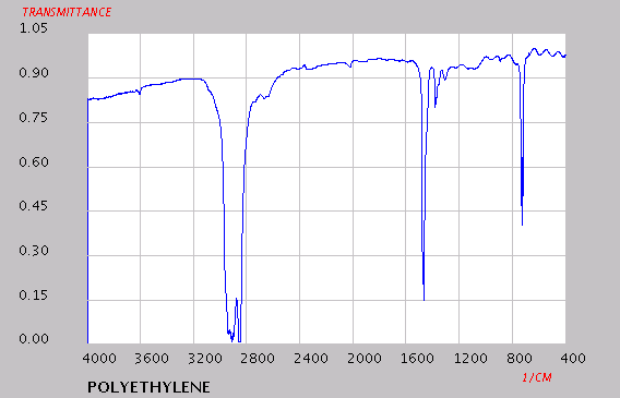
The IR Card Spectrum from The University of Arizona details three sets of peak resulting from polyethylene C-H and C-C absorption in the IR region.
 | |
|---|---|
| |
The tilt of this graph suggests that this card contains visible pigments. This source does not give a thickness for their sample; it is useful primarily for its numerical wavelength data.
The The Department of Chemistry at The University of the West Indies has an Index of IR spectra page with a polyethylene sample: "The following are some files from Tony Davies, sent as test data to check the JCAMP-DX program. They should be read without error."
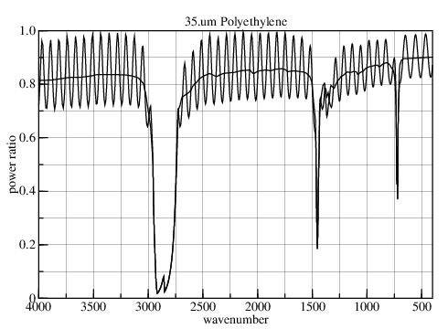
With 1800 samples, polyeth.jdx is the highest resolution data I found for polyethylene; but its utility is reduced because the transmittance is apparently scaled so its maximum is 1.0. And no description of the sample is given. Was it high or low density? How thick was the sample?
|
|---|
|
The ripples show that the sample was 35.um thick.
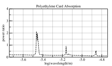
PTFE & Polyethylene IR Sample Cards from International Crystal Laboratories gives a plot of absorption by their sample cards. This is not the optical absorption, but the negative of the (natural) logarithm of the transmission through the sample, as is done in chemistry. Reflection, optical absorption, and scattering all contribute; but the graph has been corrupted so that the minimum absorption is 1 and its logarithm 0. The sample chamber of the card measures 18.um thick and is opaque white. This white pigment scatters light at the higher wavenumbers.

|
|---|
|
As one would expect of a logarithmic abscissa, the distance between 1000.cm-1 and 2000.cm-1 is the same as the distance separating 2000.cm-1 and 4000.cm-1. The distance between the ticks at 1000.cm-1 and 450.cm-1 should be more than the distance separating 1000.cm-1 and 2000.cm-1; but it isn't. The crispness of their graph indicates that video processing was done; the height of their peaks being different than modeled here could be a smoothing artifact.
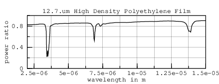
Figure 4.25 in Radiative Cooling (Martin citing Conley, R. T. 1972 "Infrared Spectroscopy", Second Edition. Boston, MA: Allyn and Bacon, Inc., p.266) is a graph of the transmission through 1/2 mil (12.7.um) HDPE from 2.um to 15.um.
|
|---|
|
Figure 4.25 has much deeper nulls than the FreeSnell simulation of 12.7.um HDPE. Its nulls are as deep as Tsilingiris's figure 2, which at 130.um thick is more than 10 times thicker! The figure 4.25 data cannot be accomodated by the model; this third-hand graph is abandoned.
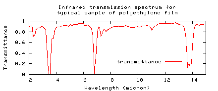
Figure 19 in Radiative cooling to low temperatures: General considerations and application to selectively emitting SiO films by Granqvist and Hjortsberg (in Journal of Applied Physics Vol 52(6) pp. 4205-4220. June 1981) is a graph of transmittance through a 14.um polyethylene film. The FreeSnell simulation of figure 19 is a good match:
|
|---|

|
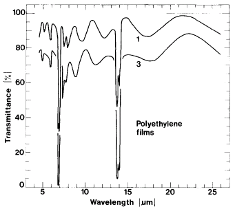
Organic Analysis - IR Theory from
California Polytechnic State University
has a graph of
low-density polyethylene
and a graph of HDPE:

|
|
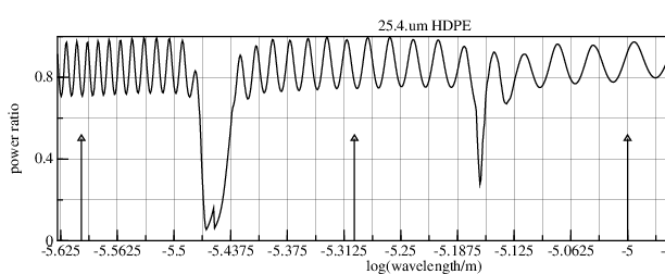
The sample thicknesses and conditions aren't disclosed. Simulating a HDPE thickness of 25.4.um (.001 inch, which is a standard thickness) gives seven peaks between the right-hand side absorption bands. But to scale the logarithmic abscissa so that the markers at 1000.cm-1, 2000.cm-1, and 4000.cm-1 are aligned, the absorption band at 735.cm-1 is pushed off the right edge!
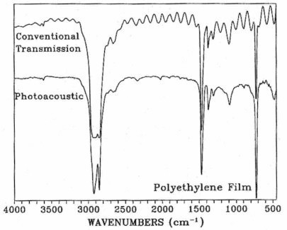
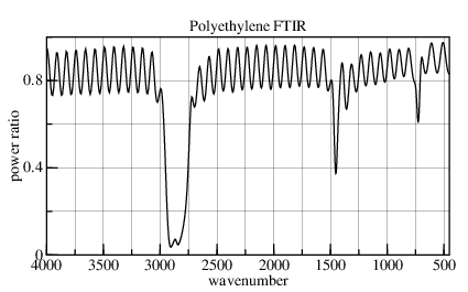
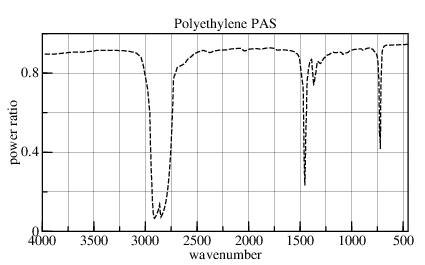
A Practical Guide to FTIR Photoacoustic Spectroscopy from MTEC Photoacoustics:
Interference fringe bands are often observed in infrared transmission spectra of polymer films. These bands interfere with and obscure important small features in spectra associated with various types of additives. FTIR-PAS spectra are free of interference artifacts due to the differences in signal generation between an absorption versus transmission based measurement.
Conventional transmission and FTIR-PAS spectra of a 32 micrometer thick polyethylene film. The PAS spectrum has been converted to transmittance for the purpose of comparison. Note the absence of interference fringes in the PAS spectrum.
While the FTIR-PAS is indeed "free of interference artifacts", it also indicates only half of the transmission changes due to variation in the real part of the refractive-index. Because different equipment generated the two plots, the video smoothing of conventional plot reduces the depth of its nulls near 735.cm-1.
Unfortunately, their graphs show only relative attenuation.
| |
|---|---|
| |
| |
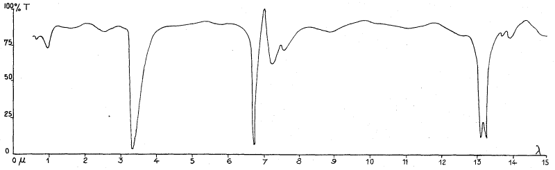
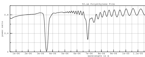
Figure 12 of Trombe's 1967 Devices for Lowering the Temperature of a Body by Heat Radiation Therefrom US Patent 3,310,102
... shows a curve indicating, in ordinates, the transparency to radiation of a polyethylene sheet of a thickness equal to 50 microns, the wavelength of the incident radiation being plotted in abscissa.
| United States Patent: 3,310,102 Figure 12. | |
|---|---|
| |
| |
| FreeSnell | |
The notch around 13.5.um is compressed in figure 12, apparently a common problem with analog spectrometers.
IR-Spectroscopy and FT-IR-Spectroscopy from the Belarussian State Technological University has "IR-Spectrums of polyethylene at various stages of ageing":
 | |
|---|---|
| |
This data this graph represents would be very important in planning for aging in radiative cooling systems if it were accompanied by details of sample age, thickness, and density, and the conditions under which they were aged.
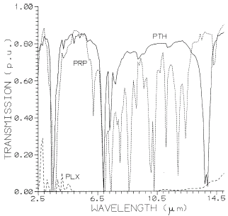
Figure 2 of Comparative evaluation of the infrared transmission of polymer films by P. T. Tsilingiris (in Energy Conversion and Management, Volume 44, Issue 18, November 2003, Pages 2839-2856) shows the transmission of a 130.um polyethylene film at wavelengths from 2.5.um to 14.9.um; the polyethylene's density is not stated. The FreeSnell simulation of figure 2 is:
|
|---|
|
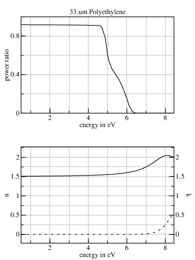
This article has a table of k-values; but the n-values must be eyeballed from a graph. The graph abscissa starts at 0.5 eV (2.48 μm) with n=1.5. The HDPE data-set ends at 2.5 μm with n=1.8+0.00016i. As a consequence, near 2.5 μm, a 33 μm thick sheet has transmission of 0.9 with the shortwave dataset versus 0.8 with the longwave one.
But it turns out that the data from 0.5 eV to 1.0 eV isn't faithful:
Below about 4.9 eV (k=10−4) k was too small to be measured using a 0.5-mil-thick sample. The use of thicker free-standing polyethylene samples (0.9-mil Glad Wrap and 4-mil Nalgene polyethylene) showed weak absorption below −1 eV but no measurable absorption from −1 to −4.5 eV.
Unable to reconcile the data around 2.5 μm, the
materials are kept separate. The shortwave refractive-index values
are in material `pe', while the longwave values are in
material `hdpe'.
|
I am a guest and not a member of the MIT Computer Science and Artificial Intelligence Laboratory.
My actions and comments do not reflect in any way on MIT. | ||
| FreeSnell | ||
| agj @ alum.mit.edu | Go Figure! | |