
|
| http://people.csail.mit.edu/jaffer/Geometry/HSFC |
Hilbert Space-Filling Curves |
Space-filling curves serve as a counterexample to less-than-rigorous notions of dimension. In addition to their mathematical importance, space-filling curves have applications to dimension reduction, mathematical programming [Butz 1968], sparse multi-dimensional database indexing [Lawder 2000], and electronics [Zhu 2003].
In 2003 I found three algorithms for the n-dimensional Hilbert Space-Filling Curve (fourth found recently):
I had some issues with these sources:
The C code in the Utah Raster Toolkit which implements Butz's algorithm does its processing through the use of computed tables.
The algorithm presented here is in terms of higher level constructs: Gray-code, lamination, rotation and reflection.
The algorithmic extension presented here is a bijection between N and Nn, imposing no limitations on integer size. Some datasets will no longer need to be scaled.
The algorithms presented here do not depend on, and are not bound by integer size limitations.

The transforms we are examining are self-similar. For the better behaved members of this class the vector displacements from changing a digit in the scalar are less than or equal to the vector displacements from changing a higher order digit.
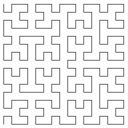
 The simplest optimal space-filling curve is one which uses two
positions on each axis.
The simplest optimal space-filling curve is one which uses two
positions on each axis.
A Gray code is an ordering of non-negative integers in
which exactly one bit differs between each pair of successive
elements. There are multiple Gray codings. An n-bit Gray code
corresponds to a Hamiltonian cycle on an n-dimensional
hypercube.
 Combining the Gray codes with self-similarity, we want the top-level
displacements to be a Gray-coded n-dimensional hypercube. To
add a layer of low-order bits, replace each stroke of the lowest-order
Gray-code with a Gray-coded hypercube.
Combining the Gray codes with self-similarity, we want the top-level
displacements to be a Gray-coded n-dimensional hypercube. To
add a layer of low-order bits, replace each stroke of the lowest-order
Gray-code with a Gray-coded hypercube.
That doesn't look right! The net displacement from each hypercube is one edge. We must rotate each small hypercube so that its net displacement matches the edge it is replacing. This series of rotations starts with the most significant hypercube.
Permutations in the n bits encoding one hypercube correspond to its rotations. When n is 2, there are only two possible rotations; but as n increases, the number of distinct rotations grows to n! (n factorial).
When there are choices in which rotation to use, the resulting curves may be different. Alber and Niedermeier [Alber 1998] reveal:
..., whereas there is basically one Hilbert curve in the 2D world, our analysis shows that there are 1536 structurally different 3D Hilbert curves.
 It turns out that cyclic rotations (shifts which loop around) of the
field of bits encoding a hypercube is sufficient for space-filling
curves.
We must also potentially reverse the net direction of the small
hypercube to match the direction of the edge it is replacing. This is
a simple matter of flipping that bit which encodes the net direction.
It turns out that cyclic rotations (shifts which loop around) of the
field of bits encoding a hypercube is sufficient for space-filling
curves.
We must also potentially reverse the net direction of the small
hypercube to match the direction of the edge it is replacing. This is
a simple matter of flipping that bit which encodes the net direction.
 The Butz algorithm and its derivatives take the number of bits per
coordinate as a parameter. Although the origin of the
multidimensional spaces are at (0, ..., 0), the coordinates returned
for other indexes depend on the width argument.
The Butz algorithm and its derivatives take the number of bits per
coordinate as a parameter. Although the origin of the
multidimensional spaces are at (0, ..., 0), the coordinates returned
for other indexes depend on the width argument.
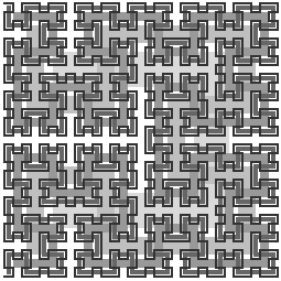
These algorithms treat their numbers as base-2 fractions; the curves generated have the same alignment independent of the width arguments. The figure to the right superimposes the curves generated for widths 1 through 5 with proportional line thicknesses. The horizontal white line is the region not covered by any of the curves.
integer->hilbert-coordinates generates these curves
when called with an optional width argument. Otherwise it treats its
scalars and coordinates as integers.
integer->hilbert-coordinates is thus a bijection from
N to Nn, imposing no limitations on
integer size.
Because the hypercube orientations are important only in relation to each other, my implementation rotates the system as a whole to an orientation such that the coordinates generated for the scalar 1 will differ from the origin in their first coordinate only. This property does not hold when calling the functions with width arguments.
integer->hilbert-coordinates is a good solution when all
the expected coordinates are nonnegative. Also useful would be a
space-filling curve covering all integer coordinates,
Zn.
Working in two dimensions, I could not find a way to orient the different sized squares so that they matched at segments around a central origin. But the base-3 Peano space-filling curve can be defined to map Z to Zn with origin at (0, ..., 0).
The integer conversions start from the high order bits, so continuing into fractional bits is straightforward. Although one can combine flonum coordinates into a scalar, as the rank grows the scalar needs more and more precision.
Perhaps the most common application of the space-filling transform is
sorting of multidimensional coordinates. D. Moore innovates by
providing box and comparison functions for rank-n floating-point
coordinates instead of floating-point Hilbert conversions
[Moore 1999].
Returns a list of rank integer coordinates corresponding to exact
non-negative integer scalar. The lists returned by integer->hilbert-coordinates for scalar arguments
0 and 1 will differ in the first element.
scalar must be a nonnegative integer of no more than
rank*k bits.
integer->hilbert-coordinates Returns a list of rank k-bit nonnegative integer
coordinates corresponding to exact non-negative integer scalar. The
curves generated by integer->hilbert-coordinates have the same alignment independent of
k.
|
I am a guest and not a member of the MIT Computer Science and Artificial Intelligence Laboratory.
My actions and comments do not reflect in any way on MIT. | ||
| Space-Filling Curves | ||
| agj @ alum.mit.edu | Go Figure! | |