
|
| http://people.csail.mit.edu/jaffer/Geometry/RMDSSF |
Recurrence for Multidimensional Self-Similar Functions |
There is a surfeit of 2-dimensional space-filling curves, but generalizing them to higher rank is not necessarily practical or even possible. [Bongki 2001] attributes generalization of space-filling curves to any rank to [Butz 1969]; who gives algorithms for the Hilbert and the Peano space-filling curves in separate papers.
Alber and Niedermeier [Alber 1998] give a mathematical description of self-similar functions; but their description is limited to functions whose self-similar units are binary (hyper)cubes. My description of the details of the multidimensional Hilbert space-filling algorithm also suffers from that limitation. Steve Witham's Hilbert Curves in More (or fewer) than Two Dimensions gives better motivation than my explanation, but is also specific to binary unit cells.
I implemented Peano Space-Filling Curves after writing about the multidimensional Hilbert space-filling algorithm. I now have a better vantage to unify the two algorithms into a single recursive formulation.
The properties we desire for space-filling transforms are that they be:
Although there are many shapes which can tile the plane, the only regular polyhedron which tiles R3 is the cube. Isotropy doesn't rule out other shapes (pyramids, for instance), but it is difficult to generalize those to all dimensions. So this article will treat the general family of curves filling squares, cubes, and hypercubes.
Because the transforms are self-similar, the scalar can be considered to be composed of digits in some base, where digits correspond to positions in nested shapes. Because transforms are measure-preserving, the largest copies of the self-similar shape correspond to the highest-order digits of the scalar.
The parameters of a space-filling function are:
Vector-valued variables and functions have uppercase names. The elements of Y are accessed as Y0, Y1, ...

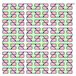
The image to the right shows two levels of the Peano Space-Filling Curve. Each of the 9 pink boxes is an instantiation of the (possibly rotated/reflected) unit Peano cell. There are 8 line segments between the 9 pink boxes. These 8 segments form another instantiation of the unit Peano cell. Let that implied cell correspond to the second tier of digits. The ninth segment connects to the top-right corner of the figure and is determined from the cell corresponding to the third tier of digits.
In each pink box is a diagonal blue arrow from the first point of its sequence to the last. This is the net travel in the pink box. For each blue arrow, there are two choices of path having the same start point and end point. In higher dimensions there are more choices. These choices distinguish the standard Peano curve from my isotropic variant.
s H(⌊x/sr⌋) is the lower-left coordinate of the unit subcell containing the point which x maps to. ⌊y⌋ is a notation for floor(y). This unit subcell must be oriented to match the entrance and exit points at each end of its blue arrow. The unit cell has entry point [0,0,...] and exit [2,2,...]. For Peano cells the entry and exit must be diagonally opposing; so we need deal only with one; without loss of generality I choose the entry point.
If the desired entry point is [0,0,...], then the unit cell can be used as is. If the desired entry point is [0,2], then the coordinates of points inside can be reflected to the desired orientation as [x0,2−x1]. Similarly, if [2,0] is desired compute [2−x0,x1]; for [2,2], compute [2−x0,2−x1]. A(U,V,s) generalizes this idea to any rank greater than 1 and to reflect cells of size s. Because Aj tests Vj only for 0, the non-zero Vj coordinates are 1.
| Aj | = Uj | when Vj = 0; | |
| Aj | = s−1−Uj | otherwise. |
N(i) is the coordinate vector of the entry corner of the subcube located at sH(i). For Peano functions, the exit corner of a subcube is opposite the entry corner; N(0) and N(sr−1) must be [0,0,...].
| 0 | if 0 = i; | |
| Nj(i−1) +1 +Hj(i)−Hj(i−1) mod 2 | otherwise. |
N(i−1) is the entry vector from the
previous subcube;
+1 is for the progression through the previous subcube.
+H(i)−H(i−1)
is for the edge between these two subcubes; and
This plot shows three levels of the Peano pattern. For this 2-dimensional Peano curve:
| i | H(i) | N(i) | |
| 0 | [0, 0] | [0, 0] | |
| 1 | [1, 0] | [0, 1] | |
| 2 | [2, 0] | [0, 0] | |
| 3 | [2, 1] | [1, 0] | |
| 4 | [1, 1] | [1, 1] | |
| 5 | [0, 1] | [1, 0] | |
| 6 | [0, 2] | [0, 0] | |
| 7 | [1, 2] | [0, 1] | |
| 8 | [2, 2] | [0, 0] |
The algorithm to convert a non-negative scalar to Peano coordinates is a tail-recursive function R. Starting with the lowest digit of x, the previously constructed coordinate vector Y is oriented according to the current digit; then added to w times H of the current digit.
| Y | if 0 = x; | |
| R( ⌊x/sr⌋, w H(x mod sr) + A(Y, N(x mod sr), w), s w ) | otherwise. |
The algorithm to convert non-negative Peano coordinates to a scalar is a tail-recursive function r. The highest digits of Y are looked up in H-1; then the rest of Y is reflected according to the entry vector N.
| r( g(Y, w) + x sr, A( [Y0 mod w, Y1 mod w, ... ], N(g(Y, w)), w), w/s ) | if 0 < w; | |
| x | otherwise. |
The plots above are anisotropic; all the straight length-5 segments are horizontal. Using a mixture of unit cells orientations could improve isotropy, even eliminate length-5 segments completely.
| rank | Y0 | Y1 | Y2 | Y3 | … | |
|---|---|---|---|---|---|---|
| ↓ | length: | 2 [=s−1] | 1 | 1 | 1 | … |
| 2 | 3 | 2 | ||||
| 3 | 9 | 6 | 2 | |||
| 4 | 27 | 18 | 6 | 2 | ||
| r | sr−1 | (s−1)⋅sr−2 | (s−1)⋅sr−3 | (s−1)⋅sr−4 | … |
The total edge length for a sr Hamiltonian-path is sr−1

There being no intrinsic distinction between axes, it makes sense to take the axes in order of decreasing edge lengths from the table above. In order to make the self-similar function isotropic, there must be equal mix of each of the r cyclic permutations of orientations. Because the function is self-similar, cells at all levels must mix orientations.
If r divides sr, then assigning successive axis permutations to subcells in H(i) order guarantees equal travel on axes while traversing scalar values 0 to integer powers of sr.
The figure to the right is a wigglier variant of the Peano curve using cyclic permutations. Because r=2 doesn't divide sr=9, there is a 2% excess of horizontal segment length versus vertical segment length (371 vs 358). This is much better than Peano's 3:1 ratio (547 horizontal vs 182 vertical). The recurrence with cyclic permutations C(Y,i) is:
| Y | if 0 = x; | |
| R( ⌊x/sr⌋ , w H(x mod sr) + A( C(Y, x mod sr) , N(x mod sr) , w ) , s w ) | otherwise. |
Segments of length 2⋅s−1 occur when the long-run axes of adjacent cells are in line with the unit segment connecting them. With the precession of cyclic-permutations, this can only occur if:
Thus length-5 runs don't happen in the rank 2 wiggly variant plot above.
The algorithm to convert non-negative iso-Peano coordinates to a scalar is a tail-recursive function r. The highest digits of Y are looked up in H-1; then the rest of Y is reflected according to the entry vector N.
| r( |
g(Y, w) + x sr, C( A( [Y0 mod w, Y1 mod w, ... ], N(g(Y, w)), w), −g(Y, w) ), w/s ) |
if 0 < w; | |
| x | otherwise. |

The image to the right shows three levels of the Hilbert Space-Filling Curve. Within a green square, each of the 4 pink boxes is an instantiation of the (possibly rotated/reflected) unit Hilbert cell. There are 3 line segments between the 4 pink boxes. These 3 segments form another instantiation of the unit Hilbert cell. Let that implied cell correspond to the second tier of digits. The sixteenth segments correspond to the third tier of digits.
The Hilbert cell is one edge short of a Hamiltonian-cycle. Thus the net progress through a cell is one edge. Furthermore, the entry and exit of each cell at each level are corners. This forces the progression (non-)edge of the first and last subcells to lie on outside edges of the cell. We can use the binary algorithm to generate the tables relating H to the subcell entry and exit corrdinates:
| i | H(i) | N(i) | X(i) | ||||
| 0 | [0, 0] | [0, 0] | [0, 1] | ||||
| 1 | [0, 1] | [0, 0] | [1, 0] | ||||
| 2 | [1, 1] | [0, 0] | [1, 0] | ||||
| 3 | [1, 0] | [1, 1] | [1, 0] |
| i | H(i) | N(i) | X(i) | ||||
| 0 | [0, 0, 0] | [0, 0, 0] | [0, 1, 0] | ||||
| 1 | [0, 1, 0] | [0, 0, 0] | [1, 0, 0] | ||||
| 2 | [1, 1, 0] | [0, 0, 0] | [1, 0, 0] | ||||
| 3 | [1, 0, 0] | [1, 1, 0] | [1, 1, 1] | ||||
| 4 | [1, 0, 1] | [1, 1, 0] | [1, 1, 1] | ||||
| 5 | [1, 1, 1] | [1, 0, 1] | [0, 0, 1] | ||||
| 6 | [0, 1, 1] | [1, 0, 1] | [0, 0, 1] | ||||
| 7 | [0, 0, 1] | [0, 1, 1] | [0, 0, 1] |
| i | H(i) | N(i) | X(i) | ||||
| 0 | [0, 0, 0, 0] | [0, 0, 0, 0] | [0, 1, 0, 0] | ||||
| 1 | [0, 1, 0, 0] | [0, 0, 0, 0] | [1, 0, 0, 0] | ||||
| 2 | [1, 1, 0, 0] | [0, 0, 0, 0] | [1, 0, 0, 0] | ||||
| 3 | [1, 0, 0, 0] | [1, 1, 0, 0] | [1, 1, 0, 1] | ||||
| 4 | [1, 0, 0, 1] | [1, 1, 0, 0] | [1, 1, 0, 1] | ||||
| 5 | [1, 1, 0, 1] | [1, 0, 0, 1] | [0, 0, 0, 1] | ||||
| 6 | [0, 1, 0, 1] | [1, 0, 0, 1] | [0, 0, 0, 1] | ||||
| 7 | [0, 0, 0, 1] | [0, 1, 0, 1] | [0, 1, 1, 1] | ||||
| 8 | [0, 0, 1, 1] | [0, 1, 0, 1] | [0, 1, 1, 1] | ||||
| 9 | [0, 1, 1, 1] | [0, 0, 1, 1] | [1, 0, 1, 1] | ||||
| 10 | [1, 1, 1, 1] | [0, 0, 1, 1] | [1, 0, 1, 1] | ||||
| 11 | [1, 0, 1, 1] | [1, 1, 1, 1] | [1, 1, 1, 0] | ||||
| 12 | [1, 0, 1, 0] | [1, 1, 1, 1] | [1, 1, 1, 0] | ||||
| 13 | [1, 1, 1, 0] | [1, 0, 1, 0] | [0, 0, 1, 0] | ||||
| 14 | [0, 1, 1, 0] | [1, 0, 1, 0] | [0, 0, 1, 0] | ||||
| 15 | [0, 0, 1, 0] | [0, 1, 1, 0] | [0, 0, 1, 0] |
The gray highlighting shows that the entry and exit coordinates repeat in pairs (i=1,2; i=3,4; ...). Geometrically, a pair of subcells act in tandem to traverse one side of the parent cell.
The difference between adjacent H values is in only one coordinate. Furthermore, that coordinate position is the only one different between the paired entry and exit coordinates. More remarkable is that the paired entry coordinates are equal to the the predecessor H value while the exit coordinates are equal to the successor H value. From these observations, the expressions for the entry and exit vectors can be written:
| N(i) = | ||||
| H( 0 ) | if i = 0; | |||
| H( 2 ⌊(i−1)/2⌋ ) | otherwise. | |||
| X(i) = | ||||
| H( sr−1 ) | if i = sr−1; | |||
| H( 1 + 2 ⌈(i+1)/2⌉ ) | otherwise. |
The reference cell is a Hamiltonian path from H(0)=[0,0,..] to a corner H(sr), having a 1 in only the hth coordinate. The goal is to transform a subcell at position i so that its entry is at the corner whose coordinates are N(i) and its exit is at the corner whose coordinates are X(i). X(i)−N(i) will be nonzero in only one coordinate, k(i), but not necessarily the same as coordinate h; swapping coordinates h and k(i) in u and conditionally complementing individual coordinates produces a satisfactory alignment.
| Aj | = Uh | when Nj(i) = 0 and j = k(i); | |
| Aj | = s−1−Uh | when Nj(i) ≠ 0 and j = k(i); | |
| Aj | = Uk(i) | when Nj(i) = 0 and j = h; | |
| Aj | = s−1−Uk(i) | when Nj(i) ≠ 0 and j = h; | |
| Aj | = Uj | when Nj(i) = 0 and j ≠ k(i) and j ≠ h; | |
| Aj | = s−1−Uj | when Nj(i) ≠ 0 and j ≠ k(i) and j ≠ h. |
| Y | if 0 = x and 0 = l; | |
| R( ⌊x/sr⌋, w H(x mod sr) + A(Y, x mod sr, w), s w, (l−1) mod r ) | otherwise. |
In two dimensions there is no wobble possible. In three or more dimensions the order of excursions parallel to the non-progressing axes can vary.
|
I am a guest and not a member of the MIT Computer Science and Artificial Intelligence Laboratory.
My actions and comments do not reflect in any way on MIT. | ||
| Space-Filling Curves | ||
| agj @ alum.mit.edu | Go Figure! | |